
Essential Math for Data Science: Scalars and Vectors
Learn the math needed for data science and machine learning using a practical approach with Python.

Machines only understand numbers. For instance, if you want to create a spam detector, you have first to convert your text data into numbers (for instance, through word embeddings). Data can then be stored in vectors, matrices, and tensors. For instance, images are represented as matrices of values between 0 and 255 representing the luminosity of each color for each pixel. It is possible to leverage the tools and concepts from the field of linear algebra to manipulate these vectors, matrices and tensors.
Linear algebra is the branch of mathematics that studies vector spaces. You’ll see how vectors constitute vector spaces and how linear algebra applies linear transformations to these spaces. You’ll also learn the powerful relationship between sets of linear equations and vector equations, related to important data science concepts like least squares approximation. You’ll finally learn important matrix decomposition methods: eigendecomposition and Singular Value Decomposition (SVD), important to understand unsupervised learning methods like Principal Component Analysis (PCA).
Scalars and Vectors
What are Vectors?
Linear algebra deals with vectors. Other mathematical entities in the field can be defined by their relationship to vectors: scalars, for example, are single numbers that scale vectors (stretching or contracting) when they are multiplied by them.
However, vectors refer to various concepts according to the field they are used in. In the context of data science, they are a way to store values from your data. For instance, take the height and weight of people: since they are distinct values with different meanings, you need to store them separately, for instance using two vectors. You can then do operations on vectors to manipulate these features without loosing the fact that the values correspond to different attributes.
You can also use vectors to store data samples, for instance, store the height of ten people as a vector containing ten values.
Notation
We’ll use lowercase, boldface letters to name vectors (such as $\vv$). As usual, refer to the Appendix in Essential Math for Data Science to have the summary of the notations used in this book.
Geometric and Coordinate Vectors
The word vector can refer to multiple concepts. Let’s learn more about geometric and coordinate vectors.
Coordinates are values describing a position. For instance, any position on earth can be specified by geographical coordinates (latitude, longitude, and elevation).
Geometric Vectors
Geometric vectors, also called Euclidean vectors, are mathematical objects defined by their magnitude (the length) and their direction. These properties allow you to describe the displacement from a location to another.
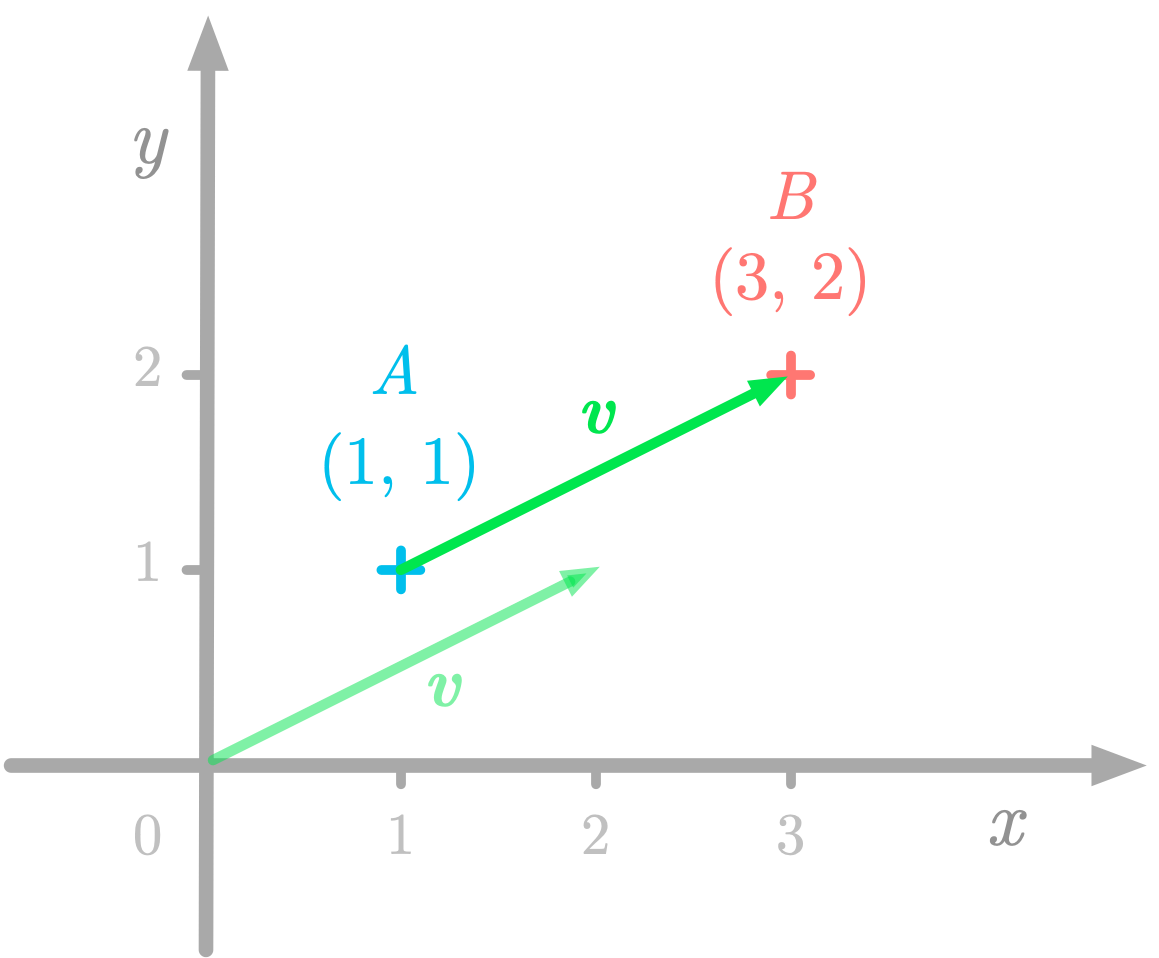 Figure 1: A geometric vector running from $A$ to $B$.
For instance, Figure 1 shows that the point $A$ has coordinates (1, 1) and the point $B$ has coordinates (3, 2). The geometric vectors $\vv$ describes the displacement from $A$ to $B$, but since vectors are defined by their magnitude and direction, you can also represent $\vv$ as starting from the origin.
In Figure 1, we used a coordinate system called the Cartesian plane. The horizontal and vertical lines are the coordinate axes, usually labeled respectively $x$ and $y$. The intersection of the two coordinates is called the origin and corresponds to the coordinate 0 for each axis.
In a Cartesian plane, any position can be specified by the $x$ and the $y$ coordinates. The Cartesian coordinate system can be extended to more dimensions: the position of a point in a $n$-dimensional space is specified by $n$ coordinates. The real coordinate $n$-dimensional space, containing $n$-tuples of real numbers, is named $\setR^n$. For instance, the space $\setR^2$ is the two-dimensional space containing pairs of real numbers (the coordinates). In three dimensions ($\setR^3$), a point in space is represented by three real numbers.
Coordinate Vectors
Coordinate vectors are ordered lists of numbers corresponding to the vector coordinates. Since vector initial points are at the origin, you need to encode only the coordinates of the terminal point.
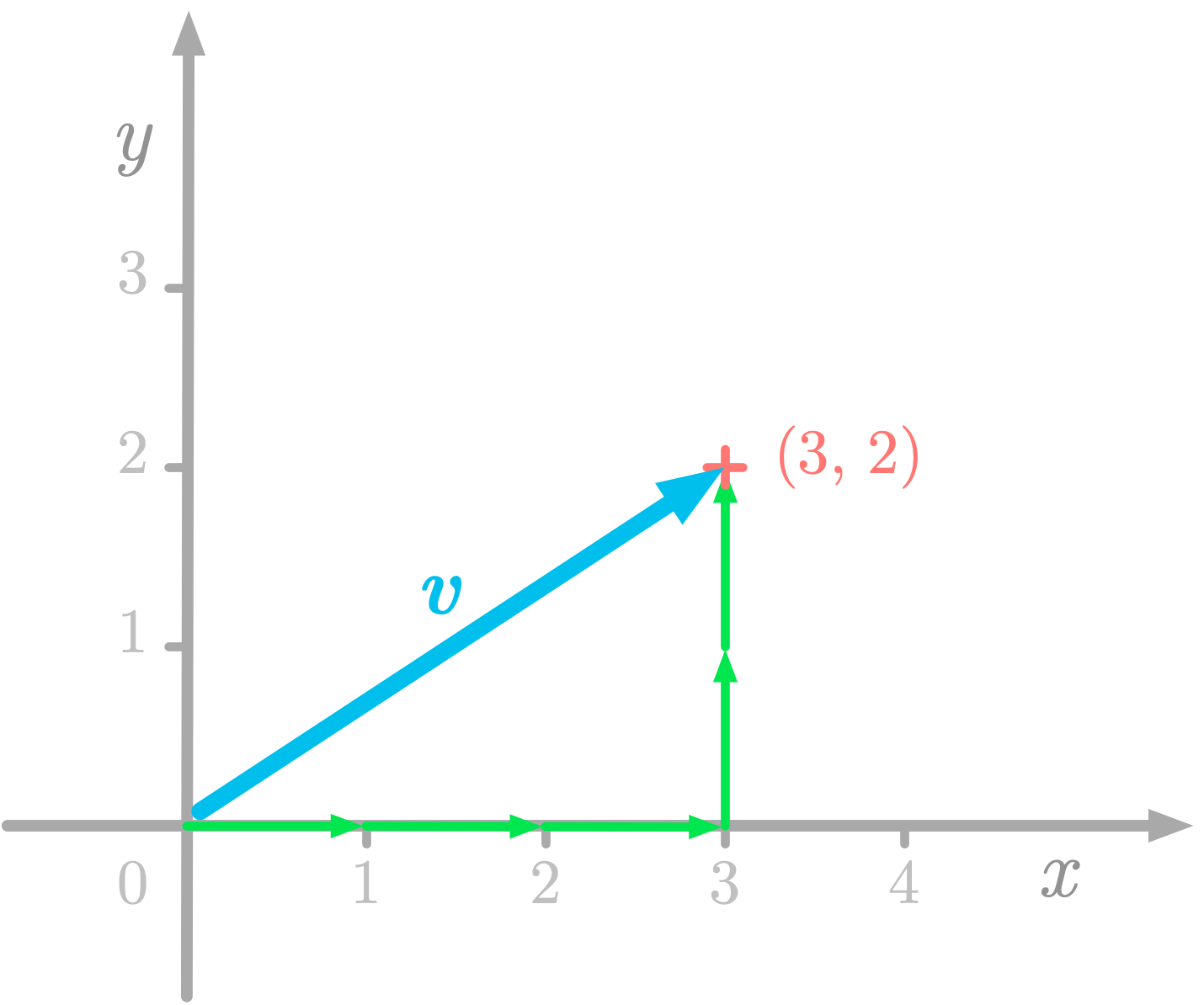 Figure 2: The vector $\vv$ has coordinates (3, 2) corresponding to three units from the origin on the $x$-axis and two on the $y$-axis.
For instance, let’s take the vector $\vv$ represented in Figure 2. The corresponding coordinate vector is as follows: \[\vv = \begin{bmatrix} 3 \\\\ 2 \end{bmatrix}\]
Each value is associated with a direction: in this case, the first value corresponds to the the $x$-axis direction and the second number to the $y$-axis.
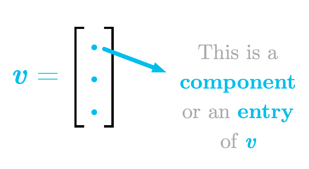 Figure 3: Components of a coordinate vector.
As illustrated in Figure 3, these values are called components or entries of the vector.
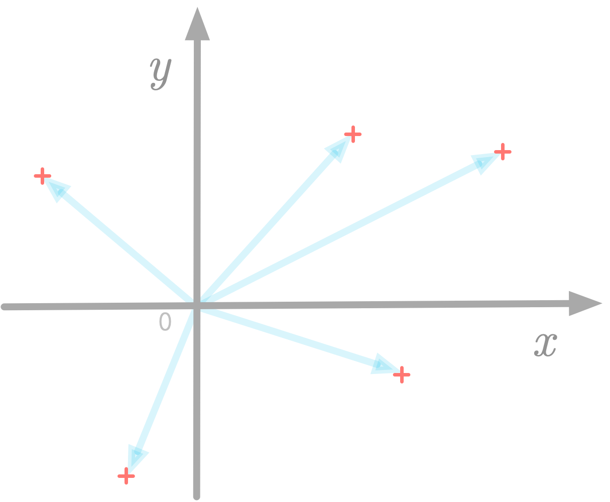 Figure 4: Vectors can be represented as points in the Cartesian plane.
In addition, as represented in Figure 4, you can simply represent the terminal point of the arrow: this is a scatter-plot.
Indexing
Indexing refers to the process of getting a vector component (one of the values from the vector) using its position (its index).
Python uses zero-based indexing, meaning that the first index is zero. However mathematically, the convention is to use one-based indexing. I’ll denote the component $i$ of the vector $\vv$ with a subscript, as $v_i$, without bold font because the component of the vector is a scalar.
Numpy
In Numpy, vectors are called one-dimensional arrays. You can use the function np.array() to create one:
v = np.array([3, 2])
v
array([3, 2])
More Components
Let’s take the example of $\vv$, a three-dimensional vectors defined as follows: \[\vv = \begin{bmatrix} 3 \\\\ 4 \\\\ 2 \end{bmatrix}\]
As shown in in Figure 5, you can reach the endpoint of the vector by traveling 3 units in the $x$-axis, 4 in the $y$-axis, and 2 in the $z$-axis.
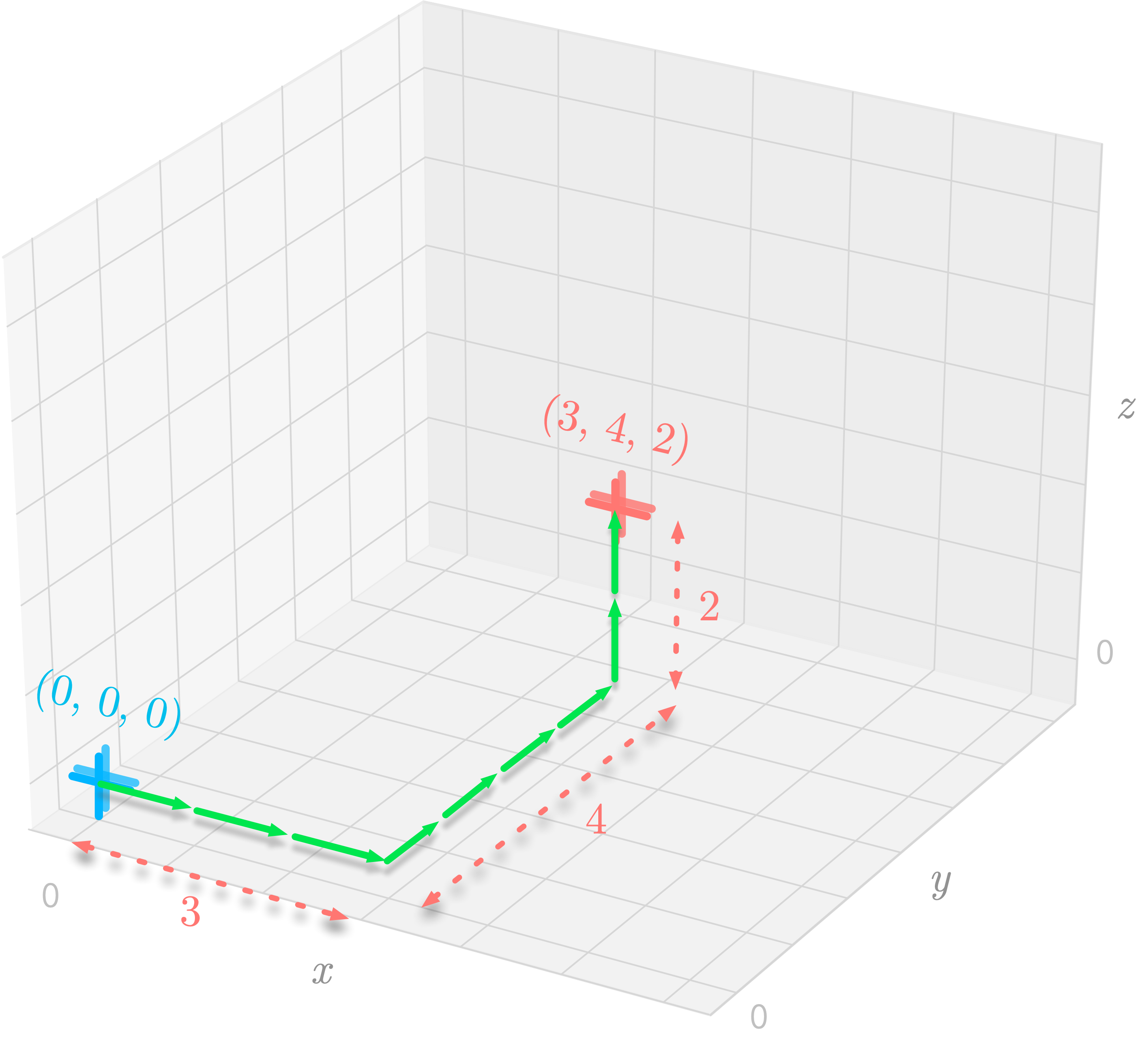 Figure 5: Three-dimensional representation of the origin at (0, 0, 0) and the point at (3, 4, 2).
More generally, in a $n$-dimensional space, the position of a terminal point is described by $n$ components.
Dimensions
You can denote the dimensionality of a vector using the set notation $\setR^n$. It expresses the real coordinate space: this is the $n$-dimensional space with real numbers as coordinate values.
For instance, vectors in $\setR^3$ have three components, as the following vector $\vv$ for example: \[\vv = \begin{bmatrix} 2.0 \\\\ 1.1 \\\\ -2.5 \end{bmatrix}\]
Vectors in Data Science
In the context of data science, you can use coordinate vectors to represent your data.
You can represent data samples as vectors with each component corresponding to a feature. For instance, in a real estate dataset, you could have a vector corresponding to an apartment with its features as different components (like the number of rooms, the location etc.).
Another way to do it is to create one vector per feature, each containing all observations.
Storing data in vectors allows you to leverage linear algebra tools. Note that, even if you can’t visualize vectors with a large number of components, you can still apply the same operations on them. This means that you can get insights about linear algebra using two or three dimensions, and then, use what you learn with a larger number of dimensions.
The Dot Product
The dot product (referring to the dot symbol used to characterize this operation), also called scalar product, is an operation done on vectors. It takes two vectors, but unlike addition and scalar multiplication, it returns a single number (a scalar, hence the name). It is an example of a more general operation called the inner product.
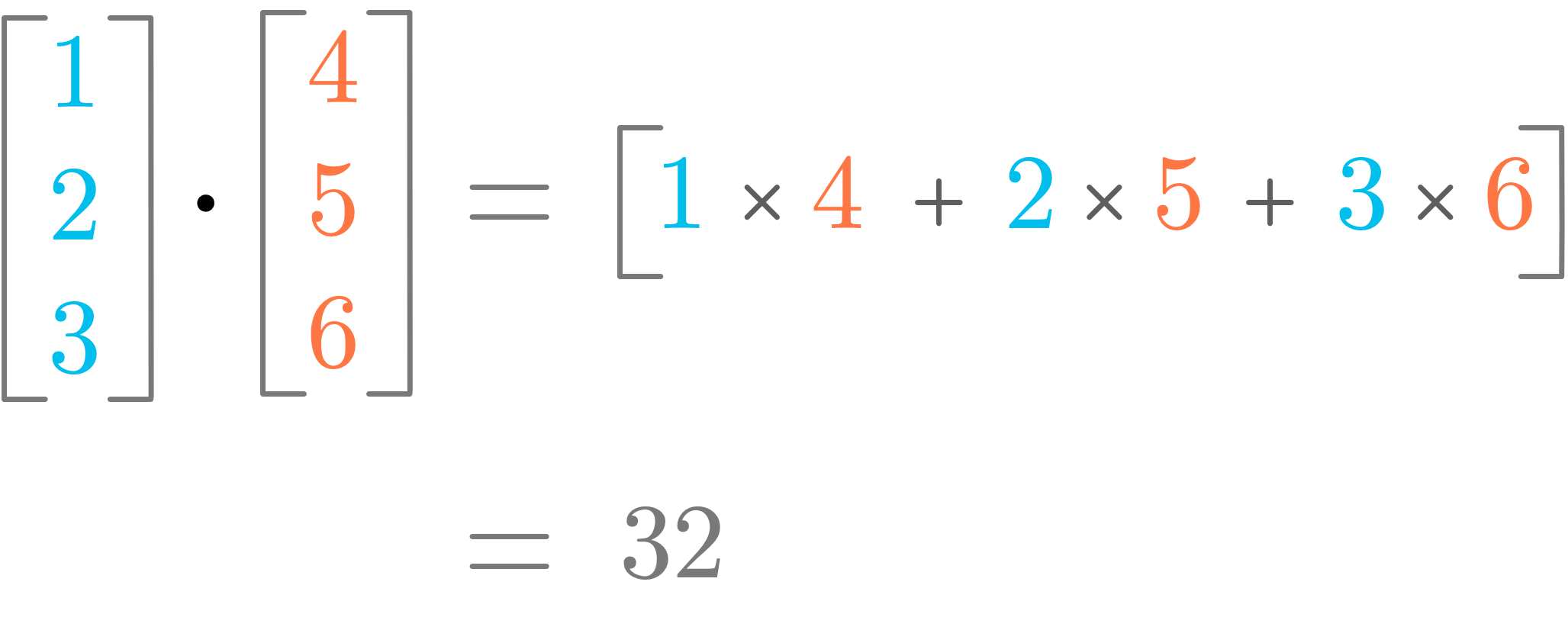 Figure 6: Illustration of the dot product.
Figure 6 shows an illustration of how the dot product works. You can see that it corresponds to the sum of the multiplication of the components with same index.
Definition
The dot product between two vectors $\vu$ and $\vv$, denoted by the symbol $\cdot$, is defined as the sum of the product of each pair of components. More formally, it is expressed as: \[\vu \cdot \vv = \sum_{i=1}^m \evu_i\evv_i\]
with $m$ the number of components of the vectors $\vu$ and $\vv$ (they must have the same number of components), and $i$ the index of the current vector component.
Note that the symbol of the dot product is the same as the dot used to refer to multiplication between scalars. The context (if the elements are scalars or vectors) tells you which one it is.
Let’s take an example. You have the following vectors: \[\vu = \begin{bmatrix} 2 \\\\ 4 \\\\ 7 \end{bmatrix}\]
and \[\vv = \begin{bmatrix} 5 \\\\ 1 \\\\ 3 \end{bmatrix}\]
The dot product of these two vectors is defined as: \[\vu \cdot \vv = \begin{bmatrix} 2 \\\\ 4 \\\\ 7 \end{bmatrix} \cdot \begin{bmatrix} 5 \\\\ 1 \\\\ 3 \end{bmatrix} = 2 \times 5 + 4 \times 1 + 7 \times 3 = 35\]
The dot product between $\vu$ and $\vv$ is 35. It converts the two vectors $\vu$ and $\vv$ into a scalar.
Let’s use Numpy to calculate the dot product of these vectors. You can use the method dot() of Numpy arrays:
u = np.array([2, 4, 7])
v = np.array([5, 1, 3])
u.dot(v)
35
It is also possible to use the following equivalent syntax:
np.dot(u, v)
35
Or, with Python 3.5+, it is also possible to use the @ operator:
u @ v
35
Note that the dot product is different from the element-wise multiplication, also called the Hadamard product, which returns another vector. The symbol $\odot$ is generally used to characterize this operation. For instance: $$ \vu \odot \vv = \begin{bmatrix} 2 \\\\ 4 \\\\ 7 \end{bmatrix} \odot \begin{bmatrix} 5 \\\\ 1 \\\\ 3 \end{bmatrix} = \begin{bmatrix} 2 \cdot 5 \\\\ 4 \cdot 1 \\\\ 7 \cdot 3 \end{bmatrix} = \begin{bmatrix} 10 \\\\ 4 \\\\ 21 \end{bmatrix} $$
Dot Product and Vector Length
The squared $L^2$ norm can be calculated using the dot product of the vector with itself ($\vu \cdot \vu$): \[\norm{\vu}_2^2 = \vu \cdot \vu\]
This is an important property in machine learning, as you saw in Essential Math for Data Science.
Special Cases
The dot product between two orthogonal vectors is equal to 0. In addition, the dot product between a unit vector and itself is equal to 1.
Geometric interpretation: Projections
How can you interpret the dot product operation with geometric vectors. You have seen in Essential Math for Data Science the geometric interpretation of the addition and scalar multiplication of vectors, but what about the dot product?
Let’s take the two following vectors: \[\vu = \begin{bmatrix} 1 \\\\ 2 \end{bmatrix}\]
and \[\vv = \begin{bmatrix} 2 \\\\ 2 \end{bmatrix}\]
First, let’s calculate the dot product of $\vu$ and $\vv$: \[\vu \cdot \vv = \begin{bmatrix} 1 \\\\ 2 \end{bmatrix} \cdot \begin{bmatrix} 2 \\\\ 2 \end{bmatrix} = 2 \cdot 1 + 2 \cdot 2 = 6\]
What is the meaning of this scalar? Well, it is related to the idea of projecting $\vu$ onto $\vv$.
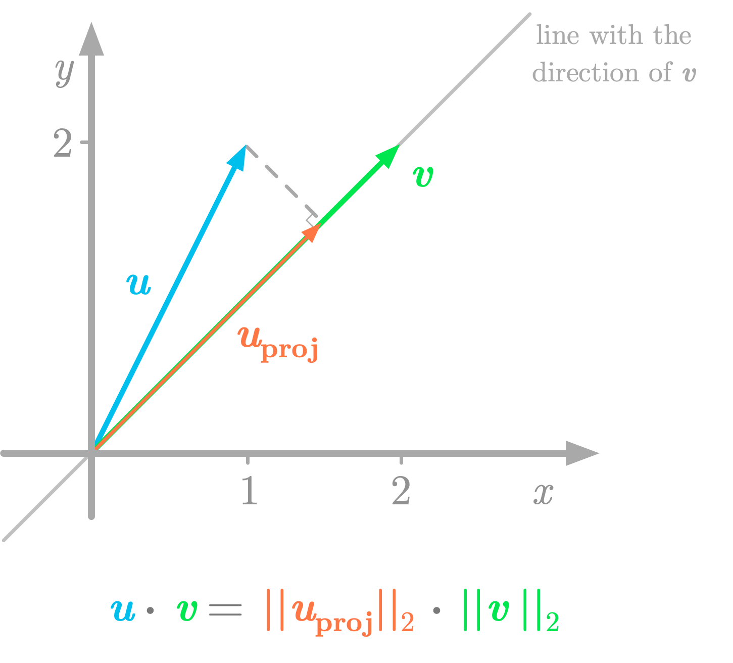 Figure 7: The dot product can be seen as the length of $\vv$ multiplied by the length of the projection (the vector $\vu_{\text{proj}}$).
As shown in Figure 7, the projection of $\vu$ on the line with the direction of $\vv$ is like the shadow of the vector $\vu$ on this line. The value of the dot product (6 in our example) corresponds to the multiplication of the length of $\vv$ (the $L^2$ norm $\norm{\vv}$) and the length of the projection of $\vu$ on $\vv$ (the $L^2$ norm $\norm{\vu_{\text{proj}}}$). You want to calculate: \[\norm{\vu_{\text{proj}}}_2 \cdot \norm{\vv}_2 \phantom{s}\]
Note that the elements are scalars, so the dot symbol refers to a multiplication of these values. And you have: \[\norm{\vv}_2 = \sqrt{2^2 + 2^2} = \sqrt{8}\]
The projection of $\vu$ onto $\vv$ is defined as follows (you can refer to Essential Math for Data Science to see the mathematical details about the projection of a vector onto a line): \[\vu_{\text{proj}} = \frac{\vu^{\text{T}}\vv}{\vv^{\text{T}}\vv}\vv = \frac{6}{8}\vv = 0.75\vv\]
So the $L^2$ norm of $\vu_{\text{proj}}$ is the $L^2$ norm of 0.75 times $\vv$: \[\norm{\vu_{\text{proj}}}_2 = 0.75 \norm{\vv}_2 = 0.75 \cdot \sqrt{8}\]
Finally, the multiplication of the length of $\vv$ and the length of the projection is: \[\norm{\vv}_2 \cdot \norm{\vu_{\text{proj}}}_2 = 0.75 \cdot \sqrt{8} \cdot \sqrt{8} = 0.75 \cdot 8 = 6\]
This shows that you can think of the dot product on geometric vectors as a projection. Using the projection gives you the same result as with the dot product formula.
Furthermore, the value that you obtain with the dot product tells you the relationship between the two vectors. If this value is positive, the angle between the vectors is less than 90 degrees, if it is negative, the angle is greater than 90 degrees, if it is zero, the vectors are orthogonal and the angle is 90 degrees.
Properties
Let’s review some properties of the dot product.
Distributive
The dot product is distributive. This means that, for instance, with the three vectors $\vu$, $\vv$ and $\vw$, you have: \[\vu \cdot (\vv + \vw) = \vu \cdot \vv + \vu \cdot \vw\]
Associative
The dot product is not associative, meaning that the order of the operations matters. For instance: \[\vu \cdot (\vv \cdot \vw) \neq (\vu \cdot \vv) \cdot \vw\]
The dot product is not a binary operator: the result of the dot product between two vectors is not another vector (but a scalar).
Commutative
The dot product between vectors is said to be commutative. This means that the order of the vectors around the dot product doesn’t matter. You have: \[\vu \cdot \vv = \vv \cdot \vu\]
However, be careful, because this is not necessarily true for matrices.
Learn the math needed for data science and machine learning using a practical approach with Python.