Introduction

This is the first post/notebook of a series following the syllabus of the linear algebra chapter from the Deep Learning Book by Goodfellow et al.. This work is a collection of thoughts/details/developements/examples I made while reading this chapter. It is designed to help you go through their introduction to linear algebra. For more details about this series and the syllabus, please see the introduction post.

This first chapter is quite light and concerns the basic elements used in linear algebra and their definitions. It also introduces important functions in Python/Numpy that we will use all along this series. It will explain how to create and use vectors and matrices through examples.

2.1 Scalars, Vectors, Matrices and Tensors

Let’s start with some basic definitions:

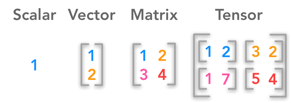An example of a scalar, a vector, a matrix and a tensor Difference between a scalar, a vector, a matrix and a tensor

A scalar is a single number
A vector is an array of numbers.

$ \bs{x} =\begin{bmatrix} x_1 \\ x_2 \\ \cdots \\ x_n \end{bmatrix} $

A matrix is a 2-D array

$ \bs{A}= \begin{bmatrix} A_{1,1} & A_{1,2} & \cdots & A_{1,n} \\ A_{2,1} & A_{2,2} & \cdots & A_{2,n} \\ \cdots & \cdots & \cdots & \cdots \\ A_{m,1} & A_{m,2} & \cdots & A_{m,n} \end{bmatrix} $

A tensor is a $n$-dimensional array with $n>2$

We will follow the conventions used in the Deep Learning Book:

scalars are written in lowercase and italics. For instance: $n$
vectors are written in lowercase, italics and bold type. For instance: $\bs{x}$
matrices are written in uppercase, italics and bold. For instance: $\bs{X}$

Example 1.

Create a vector with Python and Numpy

Coding tip: Unlike the matrix() function which necessarily creates $2$-dimensional matrices, you can create $n$-dimensionnal arrays with the array() function. The main advantage to use matrix() is the useful methods (conjugate transpose, inverse, matrix operations…). We will use the array() function in this series.

We will start by creating a vector. This is just a $1$-dimensional array:

x = np.array([1, 2, 3, 4])
x

array([1, 2, 3, 4])

Example 2.

Create a (3x2) matrix with nested brackets

The array() function can also create $2$-dimensional arrays with nested brackets:

A = np.array([[1, 2], [3, 4], [5, 6]])
A

array([[1, 2],
       [3, 4],
       [5, 6]])

Shape

The shape of an array (that is to say its dimensions) tells you the number of values for each dimension. For a $2$-dimensional array it will give you the number of rows and the number of columns. Let’s find the shape of our preceding $2$-dimensional array A. Since A is a Numpy array (it was created with the array() function) you can access its shape with:

A.shape

(3, 2)

We can see that $\bs{A}$ has 3 rows and 2 columns.

Let’s check the shape of our first vector:

x.shape

(4,)

As expected, you can see that $\bs{x}$ has only one dimension. The number corresponds to the length of the array:

len(x)

Transposition

With transposition you can convert a row vector to a column vector and vice versa:

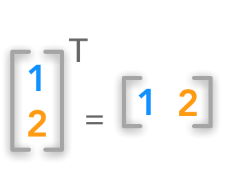Transposition of a vector Vector transposition

The transpose $\bs{A}^{\text{T}}$ of the matrix $\bs{A}$ corresponds to the mirrored axes. If the matrix is a square matrix (same number of columns and rows):

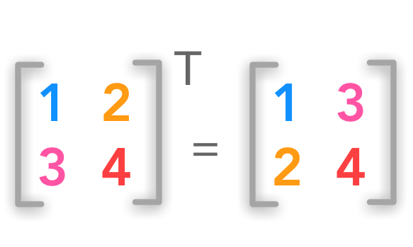Transposition of a square matrix Square matrix transposition

If the matrix is not square the idea is the same:

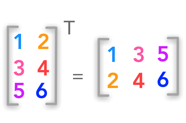Transposition of a square matrix Non-square matrix transposition

The superscript $^\text{T}$ is used for transposed matrices.

$ \bs{A}= \begin{bmatrix} A_{1,1} & A_{1,2} \\ A_{2,1} & A_{2,2} \\ A_{3,1} & A_{3,2} \end{bmatrix} $

$ \bs{A}^{\text{T}}= \begin{bmatrix} A_{1,1} & A_{2,1} & A_{3,1} \\ A_{1,2} & A_{2,2} & A_{3,2} \end{bmatrix} $

The shape ($m \times n$) is inverted and becomes ($n \times m$).

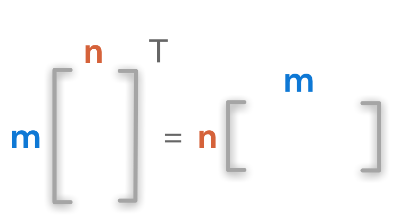Dimensions of matrix transposition

Example 3.

Create a matrix A and transpose it

A = np.array([[1, 2], [3, 4], [5, 6]])
A

array([[1, 2],
       [3, 4],
       [5, 6]])

A_t = A.T
A_t

array([[1, 3, 5],
       [2, 4, 6]])

We can check the dimensions of the matrices:

A.shape

(3, 2)

A_t.shape

(2, 3)

We can see that the number of columns becomes the number of rows with transposition and vice versa.

Addition

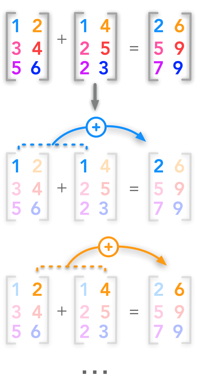Addition of two matrices

Matrices can be added if they have the same shape:

$\bs{A} + \bs{B} = \bs{C}$

Each cell of $\bs{A}$ is added to the corresponding cell of $\bs{B}$:

$\bs{A}{i,j} + \bs{B}{i,j} = \bs{C}_{i,j}$

$i$ is the row index and $j$ the column index.

$ \begin{bmatrix} A_{1,1} & A_{1,2} \\ A_{2,1} & A_{2,2} \\ A_{3,1} & A_{3,2} \end{bmatrix}+ \begin{bmatrix} B_{1,1} & B_{1,2} \\ B_{2,1} & B_{2,2} \\ B_{3,1} & B_{3,2} \end{bmatrix}= \begin{bmatrix} A_{1,1} + B_{1,1} & A_{1,2} + B_{1,2} \\ A_{2,1} + B_{2,1} & A_{2,2} + B_{2,2} \\ A_{3,1} + B_{3,1} & A_{3,2} + B_{3,2} \end{bmatrix} $

The shape of $\bs{A}$, $\bs{B}$ and $\bs{C}$ are identical. Let’s check that in an example:

Example 4.

Create two matrices A and B and add them

With Numpy you can add matrices just as you would add vectors or scalars.

A = np.array([[1, 2], [3, 4], [5, 6]])
A

array([[1, 2],
       [3, 4],
       [5, 6]])

B = np.array([[2, 5], [7, 4], [4, 3]])
B

array([[2, 5],
       [7, 4],
       [4, 3]])

# Add matrices A and B
C = A + B
C

array([[ 3,  7],
       [10,  8],
       [ 9,  9]])

It is also possible to add a scalar to a matrix. This means adding this scalar to each cell of the matrix.

$ \alpha+ \begin{bmatrix} A_{1,1} & A_{1,2} \\ A_{2,1} & A_{2,2} \\ A_{3,1} & A_{3,2} \end{bmatrix}= \begin{bmatrix} \alpha + A_{1,1} & \alpha + A_{1,2} \\ \alpha + A_{2,1} & \alpha + A_{2,2} \\ \alpha + A_{3,1} & \alpha + A_{3,2} \end{bmatrix} $

Example 5.

Add a scalar to a matrix

array([[1, 2],
       [3, 4],
       [5, 6]])

# Exemple: Add 4 to the matrix A
C = A+4
C

array([[ 5,  6],
       [ 7,  8],
       [ 9, 10]])

Broadcasting

Numpy can handle operations on arrays of different shapes. The smaller array will be extended to match the shape of the bigger one. The advantage is that this is done in C under the hood (like any vectorized operations in Numpy). Actually, we used broadcasting in the example 5. The scalar was converted in an array of same shape as $\bs{A}$.

Here is another generic example:

$ \begin{bmatrix} A_{1,1} & A_{1,2} \\ A_{2,1} & A_{2,2} \\ A_{3,1} & A_{3,2} \end{bmatrix}+ \begin{bmatrix} B_{1,1} \\ B_{2,1} \\ B_{3,1} \end{bmatrix} $

is equivalent to

$ \begin{bmatrix} A_{1,1} & A_{1,2} \\ A_{2,1} & A_{2,2} \\ A_{3,1} & A_{3,2} \end{bmatrix}+ \begin{bmatrix} B_{1,1} & B_{1,1} \\ B_{2,1} & B_{2,1} \\ B_{3,1} & B_{3,1} \end{bmatrix}= \begin{bmatrix} A_{1,1} + B_{1,1} & A_{1,2} + B_{1,1} \\ A_{2,1} + B_{2,1} & A_{2,2} + B_{2,1} \\ A_{3,1} + B_{3,1} & A_{3,2} + B_{3,1} \end{bmatrix} $

where the ($3 \times 1$) matrix is converted to the right shape ($3 \times 2$) by copying the first column. Numpy will do that automatically if the shapes can match.

Example 6.

Add two matrices of different shapes

A = np.array([[1, 2], [3, 4], [5, 6]])
A

array([[1, 2],
       [3, 4],
       [5, 6]])

B = np.array([[2], [4], [6]])
B

array([[2],
       [4],
       [6]])

# Broadcasting
C=A+B
C

array([[ 3,  4],
       [ 7,  8],
       [11, 12]])

You can find basics operations on matrices simply explained here.

References

Feel free to drop me an email or a comment. The syllabus of this series can be found in the introduction post. All the notebooks can be found on Github.

This content is part of a series following the chapter 2 on linear algebra from the Deep Learning Book by Goodfellow, I., Bengio, Y., and Courville, A. (2016). It aims to provide intuitions/drawings/python code on mathematical theories and is constructed as my understanding of these concepts. You can check the syllabus in the introduction post.