
Essential Math for Data Science: Visual Introduction to Singular Value Decomposition (SVD)
Learn the math needed for data science and machine learning using a practical approach with Python.

In this article, you’ll learn about Singular value decomposition (SVD), which is a major topic of linear algebra, data science, and machine learning. It is for instance used to calculate the Principal Component Analysis (PCA). You’ll need some understanding of linear algebra basics (feel free to check the previous article and the book Essential Math for Data Science.
You can only apply eigendecomposition to square matrices because it uses a single change of basis matrix, which implies that the initial vector and the transformed vector are relative to the same basis. You go to another basis with $\mQ$ to do the transformation, and you come back to the initial basis with $\mQ^{-1}$.
As eigendecomposition, the goal of singular value decomposition (SVD) is to decompose a matrix into simpler components: orthogonal and diagonal matrices.
You also saw that you can consider matrices as linear transformations. The decomposition of a matrix corresponds to the decomposition of the transformation into multiple sub-transformations. In the case of the SVD, the transformation is converted to three simpler transformations.
You’ll see here three examples: one in two dimensions, one comparing the transformations of the SVD and the eigendecomposition, and one in three dimensions.
Two-Dimensional Example
You’ll see the action of these transformations using a custom function matrix_2d_effect(). This function plots the unit circle (you can find more details about the unit circle in Chapter 05 of Essential Math for Data Science). and the basis vectors transformed by a matrix.
You can find the function here.
To represent the unit circle and the basis vectors before the transformation, let’s use this function using the identity matrix:
I = np.array([
    [1, 0],
    [0, 1]
])

matrix_2d_effect(I)
# [...] Add labels
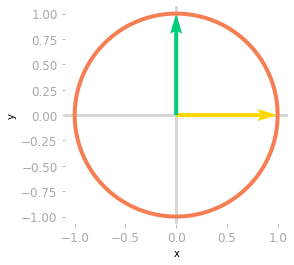 Figure 0: The unit circle and the basis vectors.
Let’s now use the function to see the effect of the following matrix $\mA$.
It will plot the unit circle and the basis vectors transformed by the matrix:
A = np.array([
    [2, 5],
    [7, 3]
])

matrix_2d_effect(A)
# [...] Add labels
 Figure 1: Effect of the matrix $\mA$ on the unit circle and the basis vectors.
Figure 1 illustrates the effect of $A$ on your two-dimensional space. Let’s compare this to the sub-transformations associated with the matrices of the SVD.
You can calculate the SVD of $\mA$ using Numpy:
U, Sigma, V_transpose = np.linalg.svd(A)
Remember that the matrices $\mU$, $\mSigma$, and $\mV$ contain respectively the left singular vectors, the singular values, and the right singular vectors. You can consider $\mV^{\text{T}}$ as a first change of basis matrix, $\mSigma$ as the linear transformation in this new basis (this transformation should be a simple scaling since $\mSigma$ is diagonal), and $\mU$ another change of basis matrix. You can see in Chapter 10 of Essential Math for Data Science that the SVD constraints both change of basis matrices $\mU$ and $\mV^{\text{T}}$ to be orthogonal, meaning that the transformations will be simple rotations.
To summarize, the transformation corresponding to the matrix $\mA$ is decomposed into a rotation (or a reflection, or a rotoreflection), a scaling, and another rotation (or a reflection, or a rotoreflection).
Let’s see the effect of each matrix successively:
matrix_2d_effect(V_transpose)
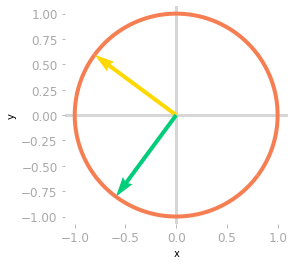 Figure 2: Effect of the matrix $\mV^{\text{T}}$ on the unit circle and the basis vectors.
You can see in Figure 2 that unit circle and the basis vectors have been rotated by the matrix $\mV^{\text{T}}$.
matrix_2d_effect(np.diag(Sigma) @ V_transpose)
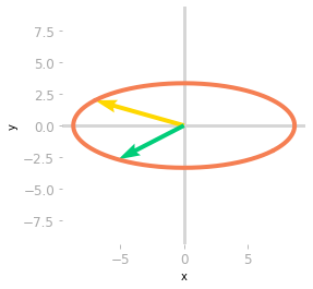 Figure 3: Effect of the matrices $\mV^{\text{T}}$ and $\mSigma$.
Then, Figure 3 shows that the effect of $\mSigma$ is a scaling of the unit circle and the basis vectors.
matrix_2d_effect(U @ np.diag(Sigma) @ V_transpose)
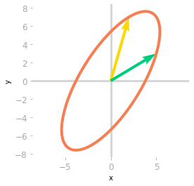 Figure 4: Effect of the matrices $\mV^{\text{T}}$, $\mSigma$ and $\mU$.
Finally, a third rotation is applied by $\mU$. You can see in Figure 4 that the transformation is the same as the one associated with the matrix $\mA$. You have decomposed the transformation into a rotation, a scaling, and a rotoreflection (look at the basis vectors: a reflection has been done because the yellow vector is on the left of the green vector, which was not the case initially).
Comparison with Eigendecomposition
Since the matrix $\mA$ was square, you can compare this decomposition with eigendecomposition and use the same type of visualization. You’ll get insights about the difference between the two methods.
Remember from Chapter 09 of Essential Math for Data Science that the eigendecomposition of the matrix $\mA$ is given by: \[\mA = \mQ \mLambda \mQ^{-1}\]
Let’s calculate the matrices $\mQ$ and $\mLambda$ (pronounced “capital lambda”) with Numpy:
lambd, Q = np.linalg.eig(A)
Note that, since the matrix $\mA$ is not symmetric, its eigenvectors are not orthogonal (their dot product is not equal to zero):
Q[:, 0] @ Q[:, 1]
-0.16609095970747995
Let’s see the effect of $\mQ^{-1}$ on the basis vectors and the unit circle:
ax = matrix_2d_effect(np.linalg.inv(Q))
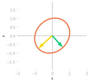 Figure 5: Effect of the matrix $\mQ^{-1}$.
You can see in Figure 5 that $\mQ^{-1}$ rotates and scales the unit circle and the basis vectors. The transformation of a non-orthogonal matrix is not a simple rotation.
The next step is to apply $\mLambda$.
ax = matrix_2d_effect(np.diag(lambd) @ np.linalg.inv(Q))
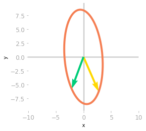 Figure 6: Effect of the matrix $\mQ^{-1}$ and $\mLambda$.
The effect of $\mLambda$, as shown in Figure 6, is a stretching and a reflection through the y-axis (the yellow vector is now on the right of the green vector).
ax = matrix_2d_effect(Q @ np.diag(lambd) @ np.linalg.inv(Q))
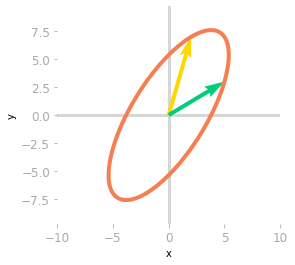 Figure 7: Effect of the matrix $\mQ^{-1}$, $\mLambda$ and $\mQ$.
The last transformation shown in Figure 7 corresponds to the change of basis back to the initial one. You can see that it leads to the same result as the transformation associated with $\mA$: both matrices $\mA$ and $\mQ \mLambda \mQ^{-1}$ are similar: they correspond to the same transformation in different bases.
It highlights the differences between eigendecomposition and SVD. With SVD, you have three different transformations, but two of them are only rotation. With eigendecomposition, there are only two different matrices, but the transformation associated with $\mQ$ is not necessarily a simple rotation (it is only the case when $\mA$ is symmetric).
Three-Dimensional Example
Since the SVD can be used with non square matrices, it is interesting to see how the transformations are decomposed in this case.
First, non square matrices map two spaces that have a different number of dimensions. Keep in mind that $m$ by $n$ matrices map an $n$-dimensional space with an $m$-dimensional space.
Let’s take the example of a 3 by 2 matrix, mapping a two-dimensional space to a three-dimensional space. This means that input vectors are two-dimensional and output vectors three-dimensional. Take the matrix $\mA$:
A = np.array([
    [2, 5],
    [1, 6],
    [7, 3]
])
To visualize the effect of $\mA$, you’ll use again the unit circle in two dimensions and calculate the output of the transformation for some points on this circle. Each point is considered as an input vector and you can observe the effect of $\mA$ on each of these vectors. The function matrix_3_by_2_effect() can be found here.
ax = matrix_3_by_2_effect(A)
# [...] Add styles axes, limits etc.
 Figure 8: Effect of the matrix $A$: it transforms vectors on the unit circle and the basis vectors from a two-dimensional space to a three-dimensional space.
As represented in Figure 8, the two-dimensional unit circle is transformed into a three-dimensional ellipse.
What you can note is that the output vectors land all on a two-dimensional plane. This is because the rank of $\mA$ is two (more details about the rank of a matrix in Section 7.6 of of Essential Math for Data Science).
Now that you know the output of the transformation by $\mA$, let’s calculate the SVD of $\mA$ and see the effects of the different matrices, as you did with the two-dimensional example.
U, Sigma, V_transpose = np.linalg.svd(A)
The shape of the left singular vectors ($\mU$) is $m$ by $m$ and the shape of the right singular vectors ($\mV^{\text{T}}$) is $n$ by $n$. There are two singular values in the matrix $\mSigma$.
The transformation associated with $\mA$ is decomposed into a first rotation in $\setR^{n}$ (associated with $\mV^{\text{T}}$, in the example, $\setR^2$), a scaling going from $\setR^{n}$ to $\setR^{m}$ (in the example, from $\setR^{2}$ to $\setR^{3}$), and a rotation in the output space $\setR^{m}$ (in the example, $\setR^{3}$).
Let’s start to inspect the effect of $\mV^{\text{T}}$ on the unit circle. You stay in two dimensions at this step:
matrix_2d_effect(V_transpose)
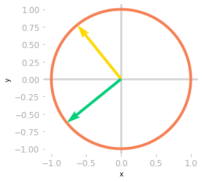 Figure 9: Effect of the matrix $\mV^{\text{T}}$: at this step, you’re still in a two-dimensional space.
You can see in Figure 9 that the basis vectors have been rotated.
Then, you need to reshape $\mSigma$ because the function np.linalg.svd() gives a one-dimensional array containing the singular values. You want a matrix with the same shape as $\mA$: a 3 by 2 matrix to go from 2D to 3D. This matrix contains the singular values as the diagonal, the other values are zero.
Let’s create this matrix:
Sigma_full = np.zeros((A.shape[0], A.shape[1]))
Sigma_full[:A.shape[1], :A.shape[1]] = np.diag(Sigma)
Sigma_full
array([[9.99274669, 0.        ],
       [0.        , 4.91375758],
       [0.        , 0.        ]])
You can now add the transformation of $\mSigma$ to see the result in 3D in Figure 10:
ax = matrix_3_by_2_effect(Sigma_full @ V_transpose)
# [...] Add styles axes, limits etc.
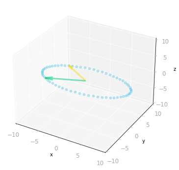 Figure 10: Effect of the matrices $\mV^{\text{T}}$ and $\mSigma$: since $\mSigma$ is a three by two matrix, it transforms two-dimensional vectors into three-dimensional vectors.
Finally, you need to operate the last change of basis. You stay in 3D because the matrix $\mU$ is a 3 by 3 matrix.
ax = matrix_3_by_2_effect(U @ Sigma_full @ V_transpose)
# [...] Add styles axes, limits etc.
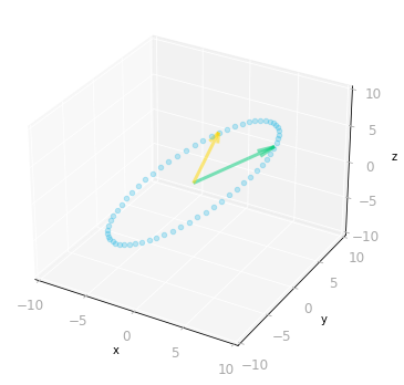 Figure 11: Effect of the three matrices $\mV^{\text{T}}$, $\mSigma$ and $\mU$: the transformation is from a three-dimensional space to a three-dimensional space.
You can see in Figure 11 that the result is identical to the transformation associated with the matrix $\mA$.
Summary
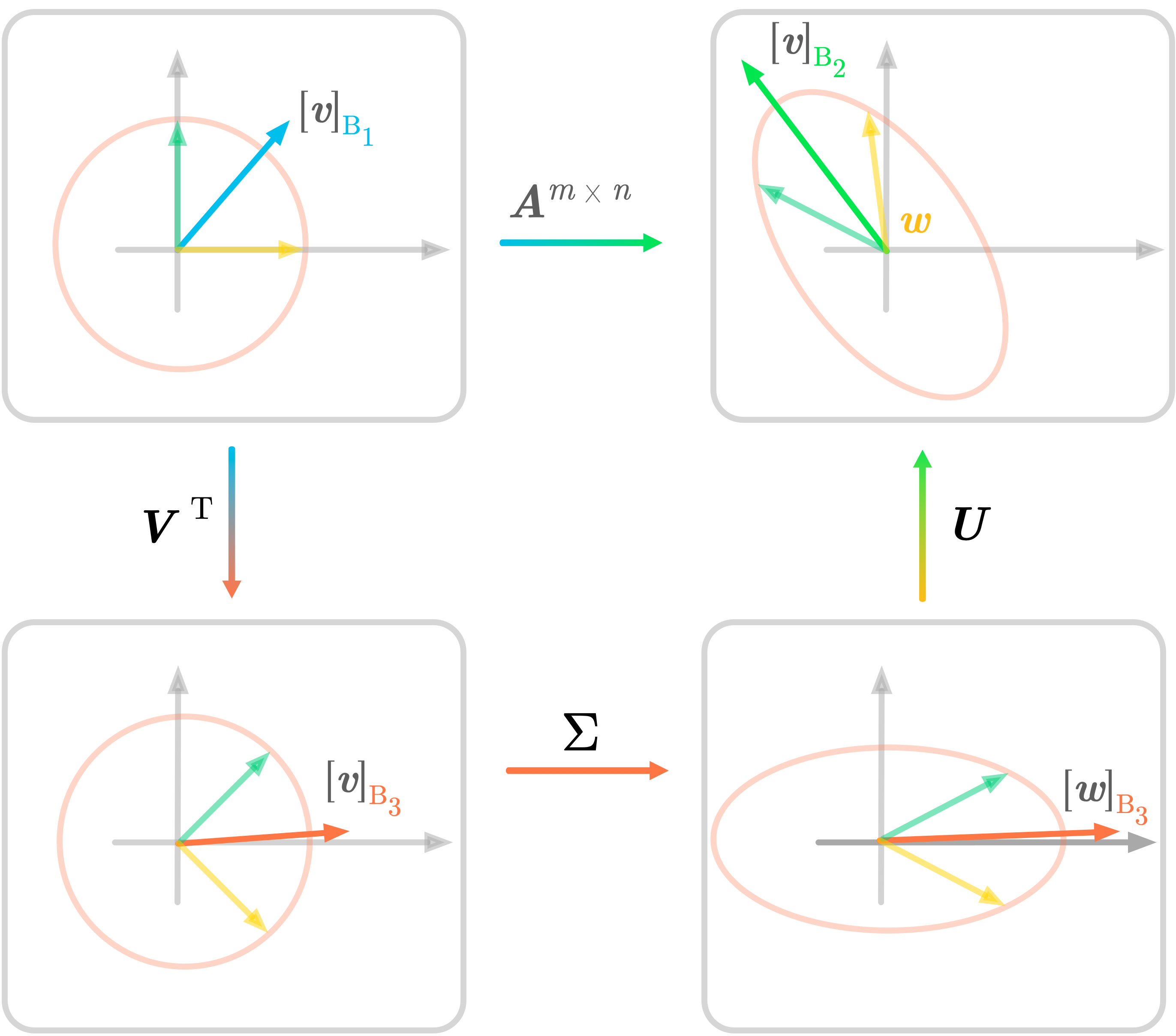 Figure 12: SVD in two dimensions.
Figure 12 summarizes the SVD decomposition of a matrix $\mA$ into three matrices. The transformation associated with $\mA$ is done by the three sub-transformations. The notation is the same as in Figure 12 and illustrates the geometric perspective of the SVD.
Singular Value Decomposition can be used for instance to find transformations that approximates well a matrix (see Low-Rank Matrix Approximation in Section 10.4 of of Essential Math for Data Science).
Learn the math needed for data science and machine learning using a practical approach with Python.