
Essential Math for Data Science: Eigenvectors and application to PCA
Learn the math needed for data science and machine learning using a practical approach with Python.

Matrix decomposition, also called matrix factorization is the process of splitting a matrix into multiple pieces. In the context of data science, you can for instance use it to select parts of the data, aimed at reducing dimensionality without losing much information (as for instance in Principal Component Analysis, as you’ll later in this post). Some operations are also more easily computed on the matrices resulting from the decomposition.
In this article, you’ll learn about the eigendecomposition of a matrix. One way to understand it is to consider it as a special change of basis (more details about change of basis in my last post). You’ll first learn about eigenvectors and eigenvalues and then you’ll see how it can be applied to Principal Component Analysis (PCA). The main idea is to consider the eigendecomposition of a matrix $\mA$ as a change of basis where the new basis vectors are the eigenvectors.
Eigenvectors and Eigenvalues
As you can see in Chapter 7 of Essential Math for Data Science you can consider matrices as linear transformations. This means that if you take any vector $\vu$ and apply the matrix $\mA$ to it, you obtain a transformed vector $\vv$.
Take the example of:
and
If you apply $\mA$ to the vector $\vu$ (with the matrix-vector product), you get a new vector:
Let’s draw the initial and transformed vectors:
u = np.array([1.5, 1])
A = np.array([
    [1.2, 0.9],
    [0, -0.4]
])
v = A @ u
plt.quiver(0, 0, u[0], u[1], color="#2EBCE7", angles='xy', scale_units='xy', scale=1)
plt.quiver(0, 0, v[0], v[1], color="#00E64E", angles='xy', scale_units='xy', scale=1)
# [...] Add axes, styles, vector names
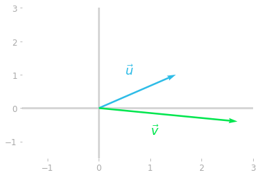 Figure 1: Transformation of the vector $\vu$ by the matrix $\mA$ into the vector $\vv$.
Note that, as you can expect, the transformed vector $\vv$ doesn’t run in the same direction as the initial vector $\vu$. This change of direction characterizes most of the vectors you can transform by $\mA$.
However, take the following vector:
Let’s apply the matrix $\mA$ to the vector $\vx$ to obtain a vector $\vy$:
x = np.array([-0.4902, 0.8715])
y = A @ x
plt.quiver(0, 0, x[0], x[1], color="#2EBCE7", angles='xy',
           scale_units='xy', scale=1)
plt.quiver(0, 0, y[0], y[1], color="#00E64E", angles='xy',
           scale_units='xy', scale=1)
# [...] Add axes, styles, vector names
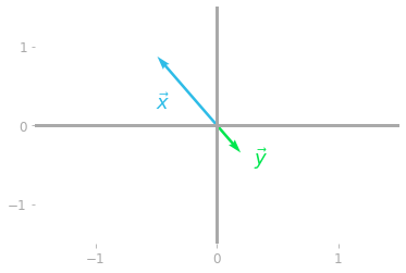 Figure 2: Transformation of the special vector $\vx$ by the matrix $\mA$.
You can see in Figure 2 that the vector $\vx$ has a special relationship with the matrix $\mA$: it is rescaled (with a negative value), but both the initial vector $\vx$ and the transformed vector $\vy$ are on the same line.
The vector $\vx$ is an eigenvector of $\mA$. It is only scaled by a value, which is called an eigenvalue of the matrix $\mA$. An eigenvector of the matrix $\mA$ is a vector that is contracted or elongated when transformed by the matrix. The eigenvalue is the scaling factor by which the vector is contracted or elongated.
Mathematically, the vector $\vx$ is an eigenvector of $\mA$ if:
with $\lambda$ (pronounced “lambda”) being the eigenvalue corresponding to the eigenvector $\vx$.
Eigenvectors of a matrix are nonzero vectors that are only rescaled when the matrix is applied to them. If the scaling factor is positive, the directions of the initial and the transformed vectors are the same, if it is negative, their directions are reversed.
Number of eigenvectors
An $n$-by-$n$ matrix has, at most, $n$ linearly independent eigenvectors. However, each eigenvector multiplied by a nonzero scalar is also an eigenvector. If you have:
Then:
with $c$ any nonzero value.
This excludes the zero vector as eigenvector, since you would have
In this case, every scalar would be an eigenvalue and thus would be undefined.
Hands-On Project: Principal Component Analysis
Principal Component Analysis, or PCA, is an algorithm that you can use to reduce the dimensionality of a dataset. It is useful, for instance, to reduce computation time, compress data, or avoid what is called the curse of dimensionality. It is also useful for visualization purposes: high dimensional data is hard to visualize and it can be useful to decrease the number of dimensions to plot your data.
In this hands-on project, you’ll use various concepts that you can learn in the book Essential Math for Data Science, as change of basis (Sections 7.5 and 9.2, some samples here), eigendecomposition (Chapter 9) or covariance matrices (Section 2.1.3) to understand how PCA is working.
In the first part, you’ll learn about the relationship between projections, explained variance and error minimization, first with a bit of theory, and then by coding a PCA on the beer dataset (consumption of beer as a function of temperature). Note that you’ll also find another example in Essential Math for Data Science where you’ll use Sklearn to use PCA on audio data to visualize audio samples according to their category, and then to compress these audio samples.
Under the Hood
Theoretical context
The goal of PCA is to project data onto a lower dimensional space while keeping as much of the information contained in the data as possible. The problem can be seen as a perpendicular least squares problem also called orthogonal regression.
You’ll see here that the error of the orthogonal projections is minimized when the projection line corresponds to the direction where the variance of the data is maximal.
Variance and Projections
It is first important to understand that, when the features of your dataset are not completely uncorrelated, some directions are associated with a larger variance than others.
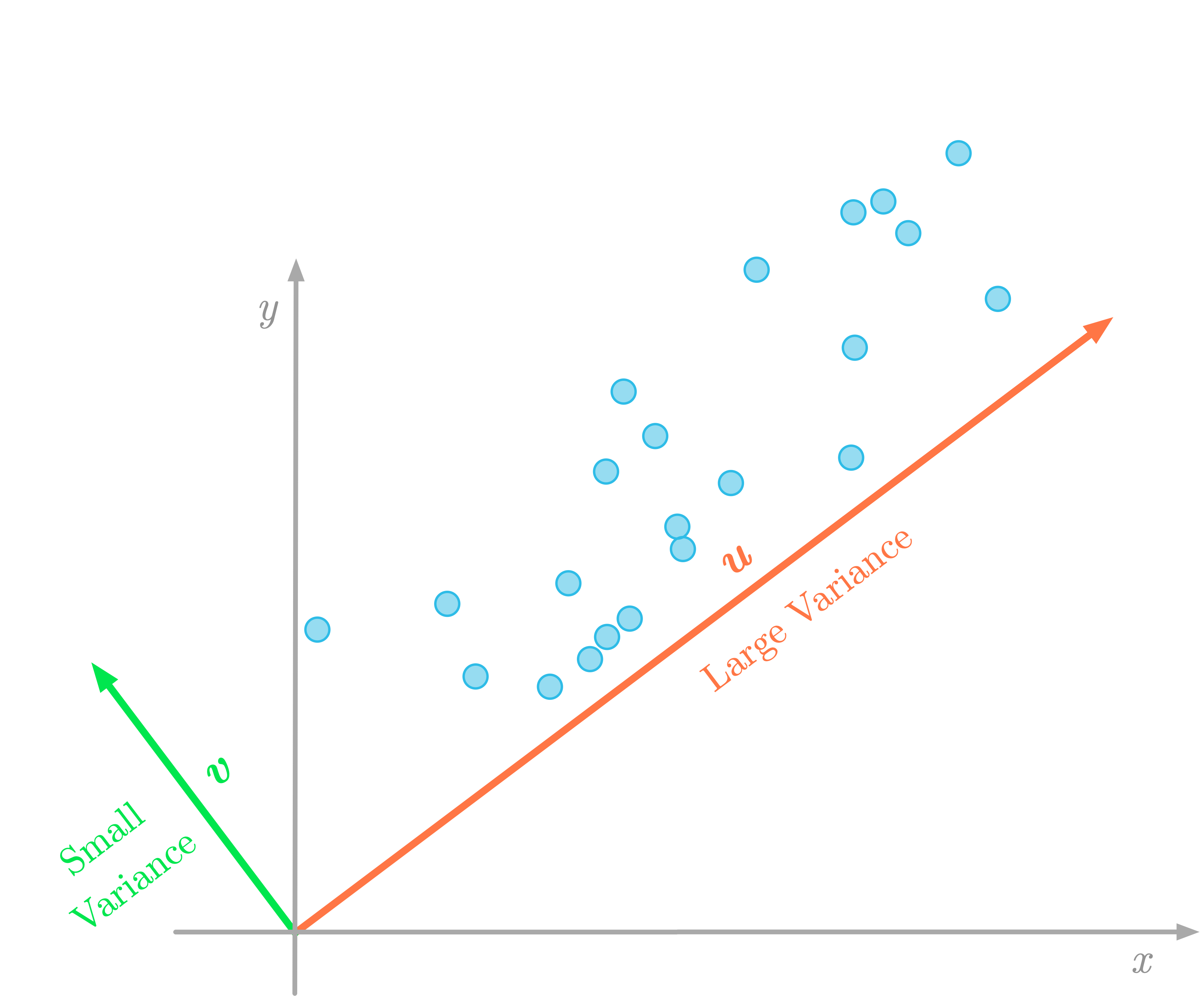 Figure 3: The variance of the data in the direction of the vector $\vu$ (red) is larger than in the direction of the vector $\vv$ (green).
Projecting data to a lower-dimensional space means that you might lose some information. In Figure 3, if you project two-dimensional data onto a line, the variance of the projected data tells you how much information you lose. For instance, if the variance of the projected data is near zero, it means that the data points will be projected to very close positions: you lose a lot of information.
For this reason, the goal of the PCA is to change the basis of the data matrix such that the direction with the maximum variance ($\vu$ in Figure 3) becomes the first principal component. The second component is the direction with the maximum variance which is orthogonal to the first one, and so on.
When you have found the components of the PCA, you change the basis of your data such that the components are the new basis vectors. This transformed dataset has new features, which are the components and which are linear combinations of the initial features. Reducing the dimensionality is done by selecting some of the components only.
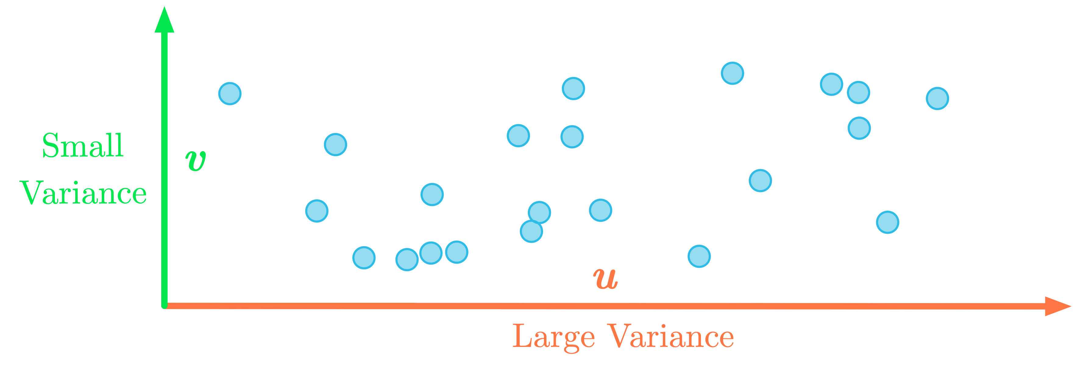 Figure 4: Change of basis such that the maximum variance is in the $x$-axis.
As an illustration, Figure 4 shows the data after a change of basis: the maximum variance is now associated with the $x$-axis. You can for instance keep only this first dimension.
In other words, expressing the PCA in terms of change of basis, its goal is to find a new basis (which is a linear combination of the initial basis) in which the variance of the data is maximized along the first dimensions.
Minimizing the Error
Finding the directions that maximize the variance is similar as minimizing the error between the data and its projection.
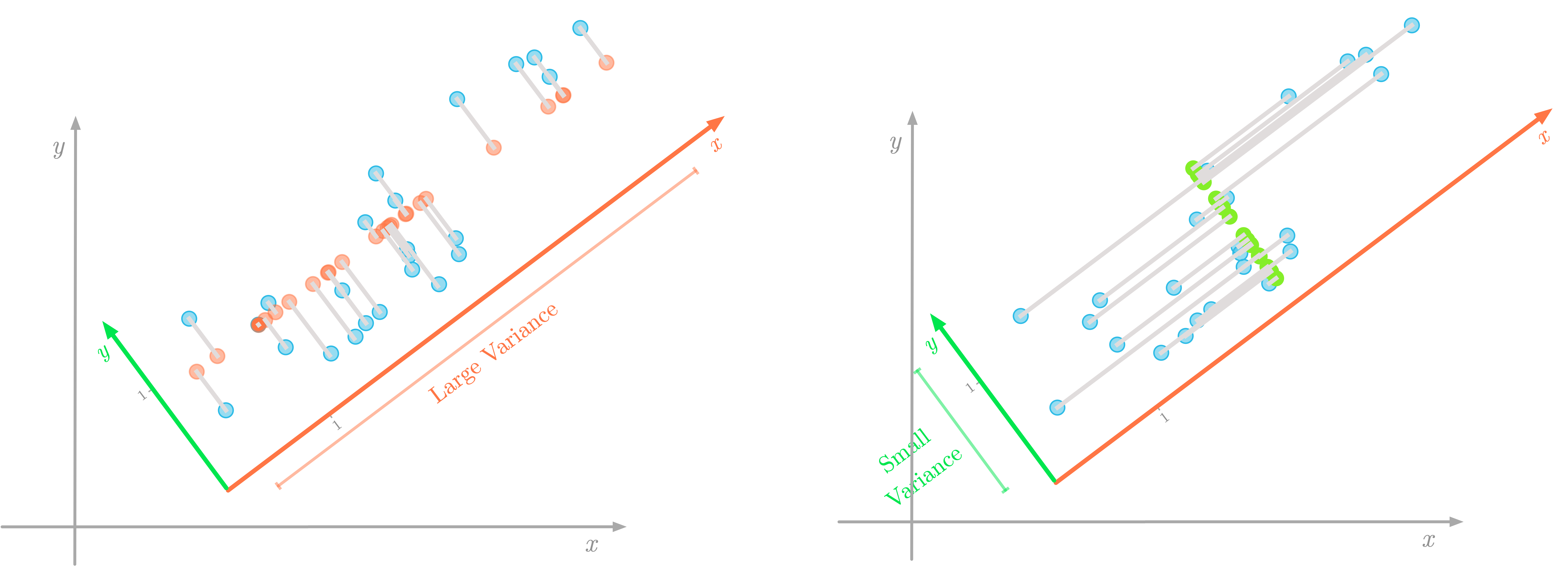 Figure 5: The direction that maximizes the variance is also the one associated with the smallest error (represented in gray).
You can see in Figure 5 that lower errors are shown in the left figure. Since projections are orthogonal, the variance associated to the direction of the line on which you project doesn’t impact the error.
Finding the Best Directions
After changing the basis of the dataset, you should have a covariance between features close to zero (as for instance in Figure 4). In other terms, you want that the transformed dataset has a diagonal covariance matrix: the covariance between each pair of principal components is equal to zero.
You can see in Chapter 9 of Essential Math for Data Science, that you can use eigendecomposition to diagonalize a matrix (make the matrix diagonal). Thus, you can calculate the eigenvectors of the covariance matrix of the dataset. They will give you the directions of the new basis in which the covariance matrix is diagonal.
To summarize, the principal components are calculated as the eigenvectors of the covariance matrix of the dataset. In addition, the eigenvalues give you the explained variance of the corresponding eigenvector. Thus, by sorting the eigenvectors in the decreasing order according to their eigenvalues, you can sort the principal components by importance order, and eventually remove the ones associated with a small variance.
Calculating the PCA
Dataset
Let’s illustrate how PCA is working with the beer dataset showing the beer consumption and the temperature in São Paulo, Brazil for the year 2015.
Let’s load the data and plot the consumption as a function of the temperature:
data_beer = pd.read_csv("https://raw.githubusercontent.com/hadrienj/essential_math_for_data_science/master/data/beer_dataset.csv")

plt.scatter(data_beer['Temperatura Maxima (C)'],
            data_beer['Consumo de cerveja (litros)'],
            alpha=0.3)
# [...] Add labels and custom axes
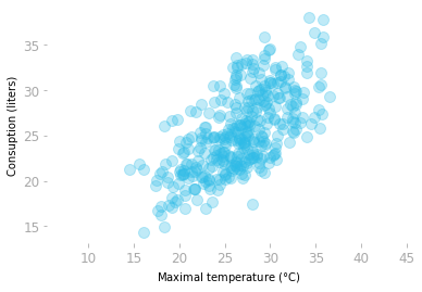 Figure 6: Consumption of beer as a function of temperature.
Now, let’s create the data matrix $\mX$ with the two variables: temperatures and consumption.
X = np.array([data_beer['Temperatura Maxima (C)'],
            data_beer['Consumo de cerveja (litros)']]).T
X.shape
(365, 2)
The matrix $\mX$ has 365 rows and two columns (the two variables).
Eigendecomposition of the Covariance Matrix
As you saw, the first step is to compute the covariance matrix of the dataset:
C = np.cov(X, rowvar=False)
C
array([[18.63964745, 12.20609082],
       [12.20609082, 19.35245652]])
Remember that you can read it as follows: the diagonal values are respectively the variances of the first and the second variable. The covariance between the two variables is around 12.2.
Now, you will calculate the eigenvectors and eigenvalues of this covariance matrix:
eigvals, eigvecs = np.linalg.eig(C)
eigvals, eigvecs
(array([ 6.78475896, 31.20734501]),
 array([[-0.71735154, -0.69671139],
        [ 0.69671139, -0.71735154]]))
You can store the eigenvectors as two vectors $\vu$ and $\vv$.
u = eigvecs[:, 0].reshape(-1, 1)
v = eigvecs[:, 1].reshape(-1, 1)
Let’s plot the eigenvectors with the data (note that you should use centered data because it is the data used to calculate the covariance matrix).
You can scale the eigenvectors by their corresponding eigenvalues, which is the explained variance. For visualization purpose, let’s use a vector length of three standard deviations (equal to three times the square root of the explained variance):
X_centered = X - X.mean(axis=0)

plt.quiver(0, 0,
           2 * np.sqrt(eigvals[0]) * u[0], 2 * np.sqrt(eigvals[0]) * u[1],
           color="#919191", angles='xy', scale_units='xy', scale=1,
           zorder=2, width=0.011)
plt.quiver(0, 0,
           2 * np.sqrt(eigvals[1]) * v[0], 2 * np.sqrt(eigvals[1]) * v[1],
           color="#FF8177", angles='xy', scale_units='xy', scale=1,
           zorder=2, width=0.011)

plt.scatter(X_centered[:, 0], X_centered[:, 1], alpha=0.3)
# [...] Add axes
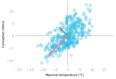 Figure 7: The eigenvectors $\vu$ (in gray) and $\vv$ (in red) scaled according to the explained variance.
You can see in Figure 7 that the eigenvectors of the covariance matrix give you the important directions of the data. The vector $\vv$ in red is associated with the largest eigenvalue and thus corresponds to the direction with the largest variance. The vector $\vu$ in gray is orthogonal to $\vv$ and is the second principal component.
Then, you just need to change the basis of the data using the eigenvectors as the new basis vectors. But first, you can sort the eigenvectors with respect to the eigenvalues in decreasing order:
sort_index = eigvals.argsort()[::-1]

eigvals_sorted = eigvals[sort_index]
eigvecs_sorted = eigvecs[:, sort_index]
eigvecs_sorted
array([[-0.69671139, -0.71735154],
       [-0.71735154,  0.69671139]])
Now that your eigenvectors are sorted, let’s change the basis of the data:
X_transformed = X_centered @ eigvecs_sorted
You can plot the transformed data to check that the principal components are now uncorrelated:
plt.scatter(X_transformed[:, 0], X_transformed[:, 1], alpha=0.3)
# [...] Add axes
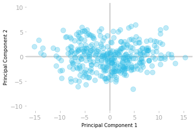 Figure 8: The dataset in the new basis.
Figure 8 shows the data samples in the new basis. You can see that the first dimension (the $x$-axis) corresponds to the direction with the largest variance.
You can keep only the first component of the data in this new basis without losing too much information.
Learn the math needed for data science and machine learning using a practical approach with Python.