
Essential Math for Data Science: Linear Transformation with Matrices
Learn the math needed for data science and machine learning using a practical approach with Python.
As you can see in Essential Math for Data Science, being able to manipulate vectors and matrices is critical to create machine learning and deep learning pipelines, for instance for reshaping your raw data before using it with machine learning libraries.
The goal of this chapter is to get you to the next level of understanding of vectors and matrices. You’ll start seeing matrices, not only as operations on numbers, but also as a way to transform vector spaces. This conception will give you the foundations needed to understand more complex linear algebra concepts like matrix decomposition. You’ll build up on what you learned about vector addition and scalar multiplication to understand linear combinations of vectors.
Linear Transformations
Intuition
A linear transformation (or simply transformation, sometimes called linear map) is a mapping between two vector spaces: it takes a vector as input and transforms it into a new output vector. A function is said to be linear if the properties of additivity and scalar multiplication are preserved, that is, the same result is obtained if these operations are done before or after the transformation. Linear functions are synonymously called linear transformations.
You can encounter the following notation to describe a linear transformation: $T(\vv)$. This refers to the vector $\vv$ transformed by $T$. A transformation $T$ is associated with a specific matrix. Since additivity and scalar multiplication must be preserved in linear transformation, you can write: $$ \tT(\vv+\vw) = \tT(\vv) + \tT(\vw) $$ and $$ \tT(c\vv) = c\tT(\vv) $$
Linear Transformations as Vectors and Matrices
In linear algebra, the information concerning a linear transformation can be represented as a matrix. Moreover, every linear transformation can be expressed as a matrix.
When you do the linear transformation associated with a matrix, we say that you apply the matrix to the vector. More concretely, it means that you calculate the matrix-vector product of the matrix and the vector. In this case, the matrix can sometimes be called a transformation matrix. For instance, you can apply a matrix $\mA$ to a vector $\vv$ with their product $\mA \vv$.
Keep in mind that, to apply a matrix to a vector, you left multiply the vector by the matrix: the matrix is on the left to the vector.
When you multiply multiple matrices, the corresponding linear transformations are combined in the order from right to left.
For instance, let's say that a matrix $\mA$ does a 45-degree clockwise rotation and a matrix $\mB$ does a stretching, the product $\mB \mA$ means that you first do the rotation and then the stretching.
This shows that the matrix product is:
- Not commutative ($\mA\mB \neq \mB\mA$): the stretching then the rotation is a different transformation than the rotation then the stretching.
- Associative ($\mA(\mB\mC)) = ((\mA\mB)\mC$): the same transformations associated with the matrices $\mA$, $\mB$ and $\mC$ are done in the same order.
A matrix-vector product can thus be considered as a way to transform a vector. You can see in Essential Math for Data Science that the shape of $\mA$ and $\vv$ must match for the product to be possible.
Geometric Interpretation
A good way to understand the relationship between matrices and linear transformations is to actually visualize these transformations. To do that, you’ll use a grid of points in a two-dimensional space, each point corresponding to a vector (it is easier to visualize points instead of arrows pointing from the origin).
Let’s start by creating the grid using the function meshgrid() from Numpy:
x = np.arange(-10, 10, 1)
y = np.arange(-10, 10, 1)

xx, yy = np.meshgrid(x, y)
The meshgrid() function allows you to create all combinations of points from the arrays x and y. Let’s plot the scatter plot corresponding to xx and yy.
plt.scatter(xx, yy, s=20, c=xx+yy)
# [...] Add axis, x and y witht the same scale
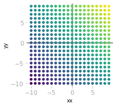 Figure 1: Each point corresponds to the combination of x and y values.
You can see the grid in Figure 1. The color corresponds to the addition of xx and yy values. This will make transformations easier to visualize.
The Linear Transformation associated with a Matrix
As a first example, let’s visualize the transformation associated with the following two-dimensional square matrix.
Consider that each point of the grid is a vector defined by two coordinates ($x$ and $y$).
Let’s create the transformation matrix $\mT$:
T = np.array([
    [-1, 0],
    [0, -1]
])
First, you need to structure the points of the grid to be able to apply the matrix to each of them. For now, you have two 20 by 20 matrices (xx and yy) corresponding to $20 \cdot 20 = 400$ points, each having a $x$ value (matrix xx) and a $y$ value (yy). Let’s create a 2 by 400 matrix with xx flatten as the first column and yy as the second column.
xy =  np.vstack([xx.flatten(), yy.flatten()])
xy.shape
(2, 400)
You have now 400 points, each with two coordinates. Let’s apply the transformation matrix $\mT$ to the first two-dimensional point (xy[:, 0]), for instance:
T @ xy[:, 0]
array([10, 10])
You can similarly apply $\mT$ to each point by calculating its product with the matrix containing all points:
trans = T @ xy
trans.shape
(2, 400)
You can see that the shape is still $(2, 400)$. Each transformed vector (that is, each point of the grid) is one of the column of this new matrix. Now, let’s reshape this array to have two arrays with a similar shape to xx and yy.
xx_transformed = trans[0].reshape(xx.shape)
yy_transformed = trans[1].reshape(yy.shape)
Let’s plot the grid before and after the transformation:
f, axes = plt.subplots(1, 2, figsize=(6, 3))
axes[0].scatter(xx, yy, s=10, c=xx+yy)
axes[1].scatter(xx_transformed, yy_transformed, s=10, c=xx+yy)
# [...] Add axis, x and y witht the same scale
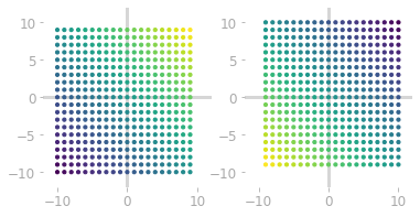 Figure 2: The grid of points before (left) and after (right) its transformation by the matrix $\mT$.
Figure 2 shows that the matrix $\mT$ rotated the points of the grid.
Shapes of the Input and Output Vectors
In the previous example, the output vectors have the same number of dimensions than the input vectors (two dimensions).
You might notice that the shape of the transformation matrix must match the shape of the vectors you want to transform.
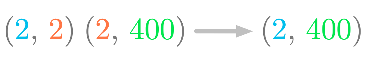 Figure 3: Shape of the transformation of the grid points by $\mT$.
Figure 3 illustrates the shapes of this example. The first matrix with a shape (2, 2) is the transformation matrix $\mT$ and the second matrix with a shape (2, 400) corresponds to the 400 vectors stacked. As illustrated in blue, the number of rows of the $\mT$ corresponds to the number of dimensions of the output vectors. As illustrated in red, the transformation matrix must have the same number of columns as the number of dimensions of the matrix you want to transform.
More generally, the size of the transformation matrix tells you the input and output dimensions. An $m$ by $n$ transformation matrix transforms $n$-dimensional vectors to $m$-dimensional vectors.
Stretching and Rotation
Let’s now visualize the transformation associated with the following matrix:
Let’s proceed as in the previous example:
T = np.array([
    [1.3, -2.4],
    [0.1, 2]
])
trans = T @ xy

xx_transformed = trans[0].reshape(xx.shape)
yy_transformed = trans[1].reshape(yy.shape)

f, axes = plt.subplots(1, 2, figsize=(6, 3))
axes[0].scatter(xx, yy, s=10, c=xx+yy)
axes[1].scatter(xx_transformed, yy_transformed, s=10, c=xx+yy)
# [...] Add axis, x and y witht the same scale
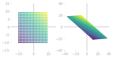 Figure 4: The grid of points before (left) and after (right) the transformation by the new matrix $\mT$.
Figure 4 shows that the transformation is different from the previous rotation. This time, there is a rotation, but also a stretching of the space.
You might wonder why these transformations are called "linear". You saw that a linear transformation implies that the properties of additivity and scalar multiplication are preserved.
Geometrically, there is linearity if the vectors lying on the same line in the input space are also on the same line in the output space, and if the origin remains at the same location.
Special Cases
Inverse Matrices
Transforming the space with a matrix can be reversed if the matrix is invertible. In this case, the inverse $\mT^{-1}$ of the matrix $\mT$ is associated with a transformation that takes back the space to the initial state after $\mT$ has been applied.
Let’s take again the example of the transformation associated with the following matrix:
You’ll plot the initial grid of point, the grid after being transformed by $\mT$, and the grid after successive application of $\mT$ and $\mT^{-1}$ (remember that matrices must be left-multiplied):
T = np.array([
    [1.3, -2.4],
    [0.1, 2]
])
trans = T @ xy

T_inv = np.linalg.inv(T)

un_trans = T_inv @ T @ xy

f, axes = plt.subplots(1, 3, figsize=(9, 3))
axes[0].scatter(xx, yy, s=10, c=xx+yy)
axes[1].scatter(trans[0].reshape(xx.shape), trans[1].reshape(yy.shape), s=10, c=xx+yy)
axes[2].scatter(un_trans[0].reshape(xx.shape), un_trans[1].reshape(yy.shape), s=10, c=xx+yy)

# [...] Add axis, x and y witht the same scale
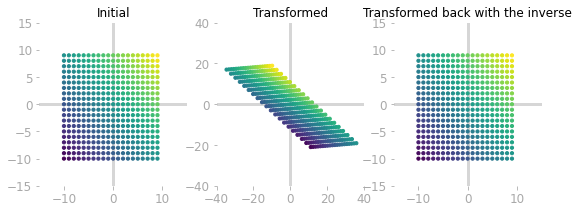 Figure 5: Inverse of a transformation: the initial space (left) is transformed with the matrix $\mT$ (middle) and transformed back using $\mT^{-1}$ (right).
As you can see in Figure 5, the inverse $\mT^{-1}$ of the matrix $\mT$ is associated with a transformation that reverses the one associated with $\mT$.
Mathematically, the transformation of a vector $\vv$ by $\mT$ is defined as: \[\mT \vv\]
To transform it back, you multiply by the inverse of $\mT$: \[\mT^{-1} \mT \vv\]
Note that the order of the products is from right to left. The vector on the right of the product is first transformed by $\mT$ and then the result is transformed by $\mT^{-1}$.
As you can see in Essential Math for Data Science, $\mT^{-1} \mT = \mI$, so you have: \[\mT^{-1} \mT \vv = \mI \vv = \vv\]
meaning that you get back the initial vector $\vv$.
Non Invertible Matrices
The linear transformation associated with a singular matrix (that is a non invertible matrix) can’t be reversed. It can occur when there is a loss of information with the transformation. Take the following matrix:
Let’s see how it transforms the space:
T = np.array([
    [3, 6],
    [2, 4],
])
trans = T @ xy

f, axes = plt.subplots(1, 2, figsize=(6, 3))
axes[0].scatter(xx, yy, s=10, c=xx+yy)
axes[1].scatter(trans[0].reshape(xx.shape), trans[1].reshape(yy.shape), s=10, c=xx+yy)
# [...] Add axis, x and y witht the same scale
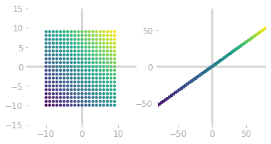 Figure 6: The initial space (left) is transformed into a line (right) with the matrix $\mT$. Multiple input vectors land on the same location in the output space.
You can see in Figure 6 that the transformed vectors are on a line. There are points that land on the same place after the transformation. Thus, it is not possible to go back. In this case, the matrix $\mT$ is not invertible: it is singular.
Learn the math needed for data science and machine learning using a practical approach with Python.