
Essential Math for Data Science: Introduction to Systems of Linear Equations
Learn the math needed for data science and machine learning using a practical approach with Python.

Systems of Linear Equations
In this article, you’ll be able to use what you learned about vectors and matrices, and linear combinations (respectively Chapter 05, 06 and 07 of Essential Math for Data Science). This will allow you to convert data into systems of linear equations. At the end of this chapter (in Essential Math for Data Science), you’ll see how you can use systems of equations and linear algebra to solve a linear regression problem.
Linear equations are formalizations of the relationship between variables. Take the example of a linear relationship between two variables $x$ and $y$ defined by the following equation:
You can represent this relationship in a Cartesian plane:
# create x and y vectors
x = np.linspace(-2, 2, 100)
y = 2 * x + 1
plt.plot(x, y)
# [...] Add axes and styles
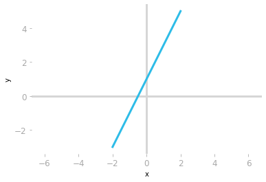 Figure 1: Plot of the equation $y=2x+1$.
Remember that each point on the line corresponds to a solution of this equation: if you replace $x$ and $y$ with the coordinates of a point on the line in this equation, the equality is satisfied. This means that there is an infinite number of solutions (every point in the line).
It is also possible to consider more than one linear equation using the same variables: this is a system of equations.
System of linear equations
A system of equations is a set of equations describing the relationship between variables. For instance, let’s consider the following example:
You have two linear equations and they both characterize the relationship between the variables $x$ and $y$. This is a system with two equations and two variables (also called unknowns in this context).
You can consider systems of linear equations (each row of the system) as multiple equations, each corresponding to a line. This is called the row picture.
You can also consider the system as different columns corresponding to coefficients scaling the variables. This is called the column picture. Let’s see more details about these two pictures.
Row Picture
With the row picture, each row of the system corresponds to an equation. In the previous example, there are two equations describing the relationship between two variables $x$ and $y$.
Graphical Representation of the Row Picture
Let’s represent the two equations graphically:
# create x and y vectors
x = np.linspace(-2, 2, 100)
y = 2 * x + 1
y1 = -0.5 * x + 3
plt.plot(x, y)
plt.plot(x, y1)
# [...]
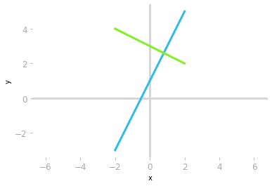 Figure 2: Representation of the two equations from our system.
Having more than one equation means that the values of $x$ and $y$ must satisfy more equations. Remember that the $x$ and $y$ from the first equation are the same as the $x$ and $y$ from the second equation.
All points on the blue line satisfy the first equation and all points on the green line satisfy the second equation. This means that only the point on both lines satisfies the two equations. The system of equations is solved when $x$ and $y$ take the values corresponding to the coordinates of the line intersection.
In this example, this point has an $x$-coordinate of 0.8 and a $y$-coordinate of 2.6. If you replace these values in the system of equations, you have:
This is a geometrical way of solving the system of equations. The linear system is solved for $x=0.8$ and $y=2.6$.
Column Picture
Viewing the system as columns is called the column picture: you consider your system as unknown values ($x$ and $y$) that scale vectors.
To better see this, let’s rearrange the equations to have the variables on one side and the constants on the other side. For the first, you have:
and for the second:
You can now write the system as:
You can now look at Figure 3 to see how to convert the two equations into a single vector equation.
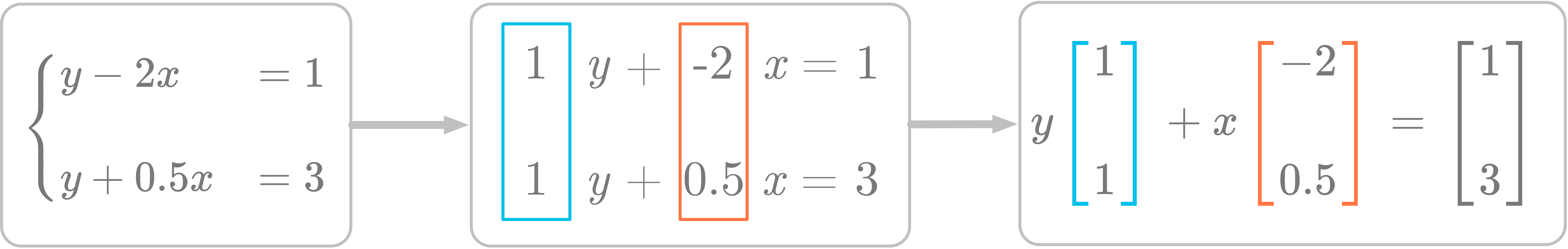 Figure 3: Considering the system of equations as column vectors scaled by the variables $x$ and $y$.
On the right of Figure 3, you have the vector equation. There are two column vectors on the left-hand side and one column vector on the right-hand side. As you saw in Essential Math for Data Science, this corresponds to a linear combination of the following vectors:
and
With the column picture, you replace multiple equations with a single vector equation. In this perspective, you want to find the linear combination of the left-hand side vectors that gives you the right-hand side vector.
The solution in the column picture is the same. Row and column pictures are just two different ways to consider the system of equations:
It works: you get the right-hand side vector if you use the solution you found geometrically.
Graphical Representation of the Column Picture
Let’s represent the system of equations considering it as a linear combination of vectors. Let’s take again the previous example:
Figure 4 shows the graphical representation of the two vectors from the left-hand side (the vectors you want to combine, in blue and red in the picture) and the vector from the right-hand side of the equation (the vector you want to obtain from the linear combination, in green in the picture).
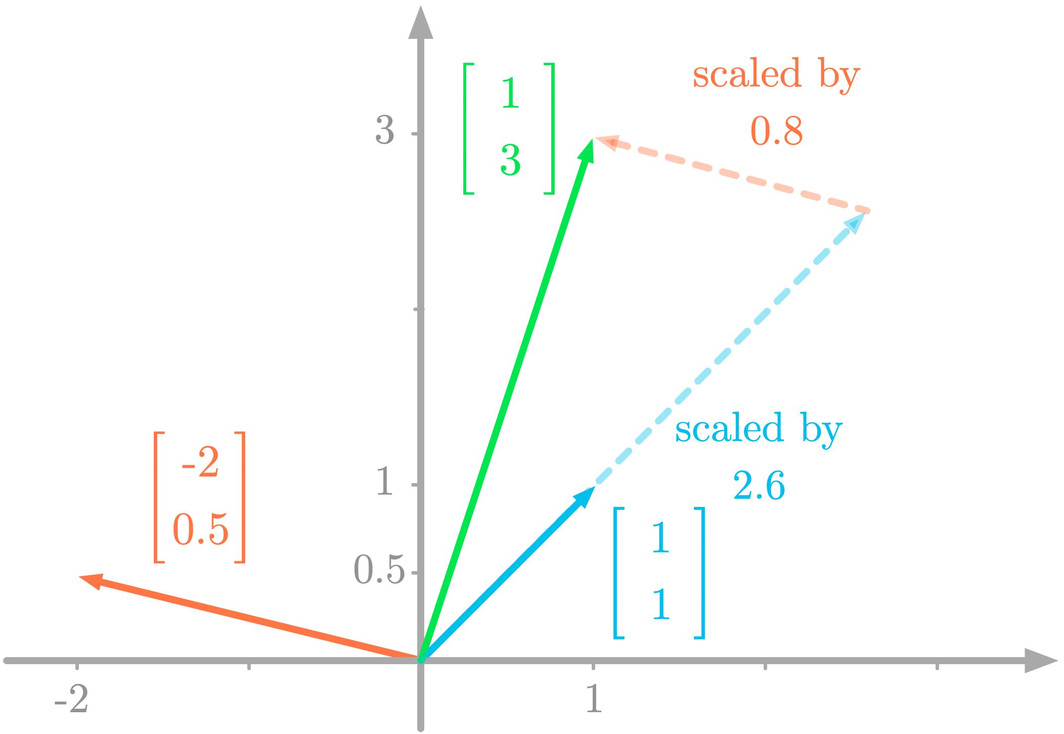 Figure 4: Linear combination of the vectors scaled by $x$ and $y$ gives the right-hand vector.
You can see in Figure 4 that you can reach the right-hand side vector by combining the left-hand side vectors. If you scale the vectors with the values 2.6 and 0.8, the linear combination gets you to the vector on the right-hand side of the equation.
Number of Solutions
In some linear systems, there is not a unique solution. Actually, linear systems of equations can have either:
- No solution.
- One solution.
- An infinite number of solutions.
Let’s consider these three possibilities (with the row picture and the column picture) to see how it is impossible for a linear system to have more than one solution and less than an infinite number of solutions.
Example 1. No Solution
Let’s take the following linear system of equations, still with two equations and two variables:
We’ll start by representing these equations:
# create x and y vectors
x = np.linspace(-2, 2, 100)
y = 2 * x + 1
y1 = 2 * x + 3

plt.plot(x, y)
plt.plot(x, y1)
# [...] Add axes, styles...
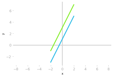 Figure 5: Parallel equation lines.
As you can see in Figure 5, there is no point that is on both the blue and green lines. This means that this system of equations has no solution.
You can also understand graphically why there is no solution through the column picture. Let’s write the system of equations as follows:
Writing it as a linear combination of column vectors, you have:
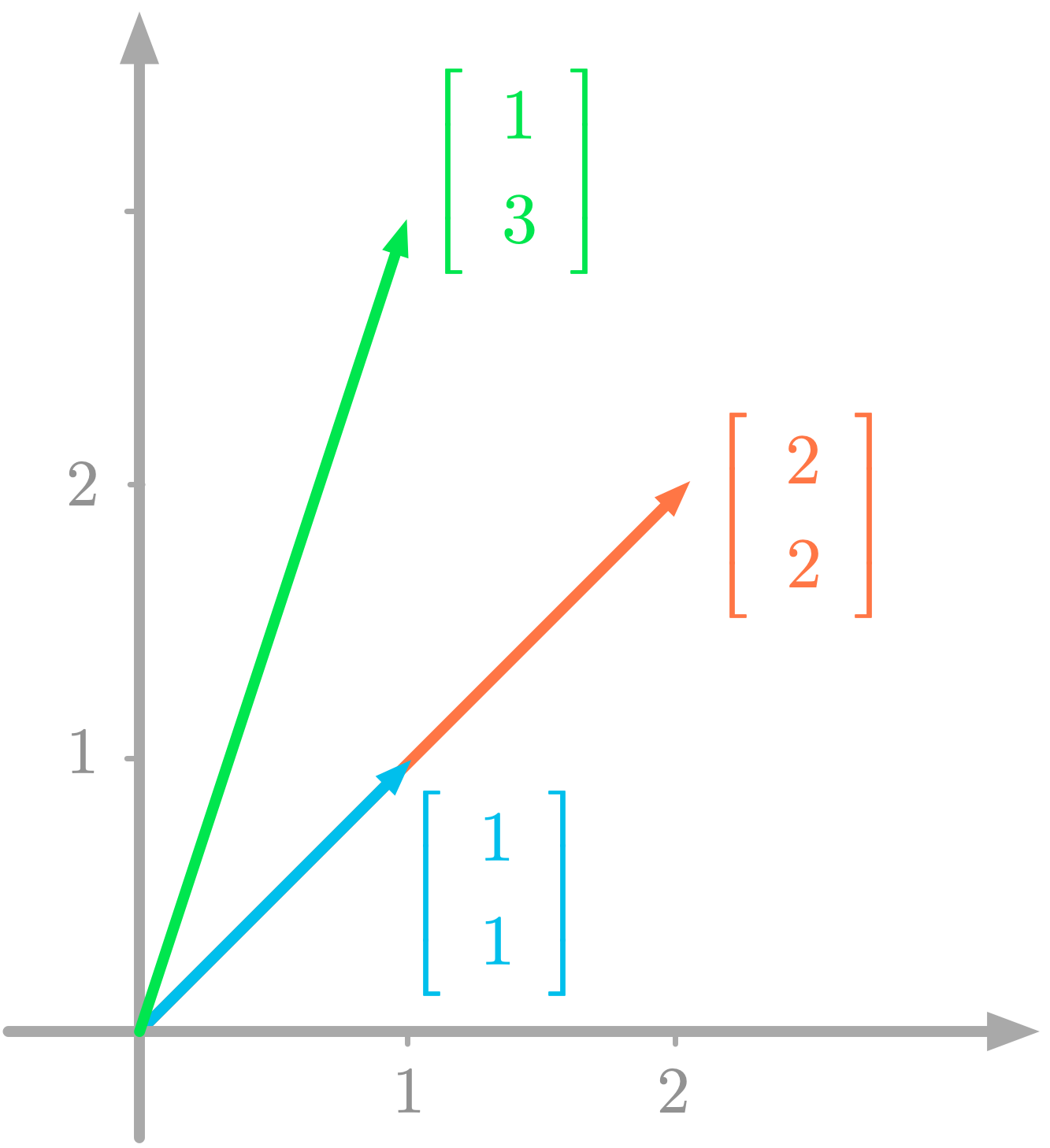 Figure 6: Column picture of a linear system with no solution.
Figure 6 shows the column vectors of the system. You can see that it is impossible to reach the endpoint of the green vector by combining the blue and the red vectors. The reason is that these vectors are linearly dependent (more details in Essential Math for Data Science). The vector to reach is outside of the span of the vectors you combine.
Example 2. Infinite Number of Solutions
You can encounter another situation where the system has an infinite number of solutions. Let’s consider the following system:
# create x and y vectors
x = np.linspace(-2, 2, 100)
y = 2 * x + 1
y1 = (4 * x + 2) / 2

plt.plot(x, y)
plt.plot(x, y1, alpha=0.3)
# [...] Add axes, styles...
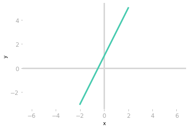 Figure 7: The equation lines are overlapping.
Since the equations are the same, an infinite number of points are on both lines and thus, there is an infinite number of solutions for this system of linear equations. This is for instance similar to the case with a single equation and two variables.
From the column picture perspective, you have:
and with the vector notation:
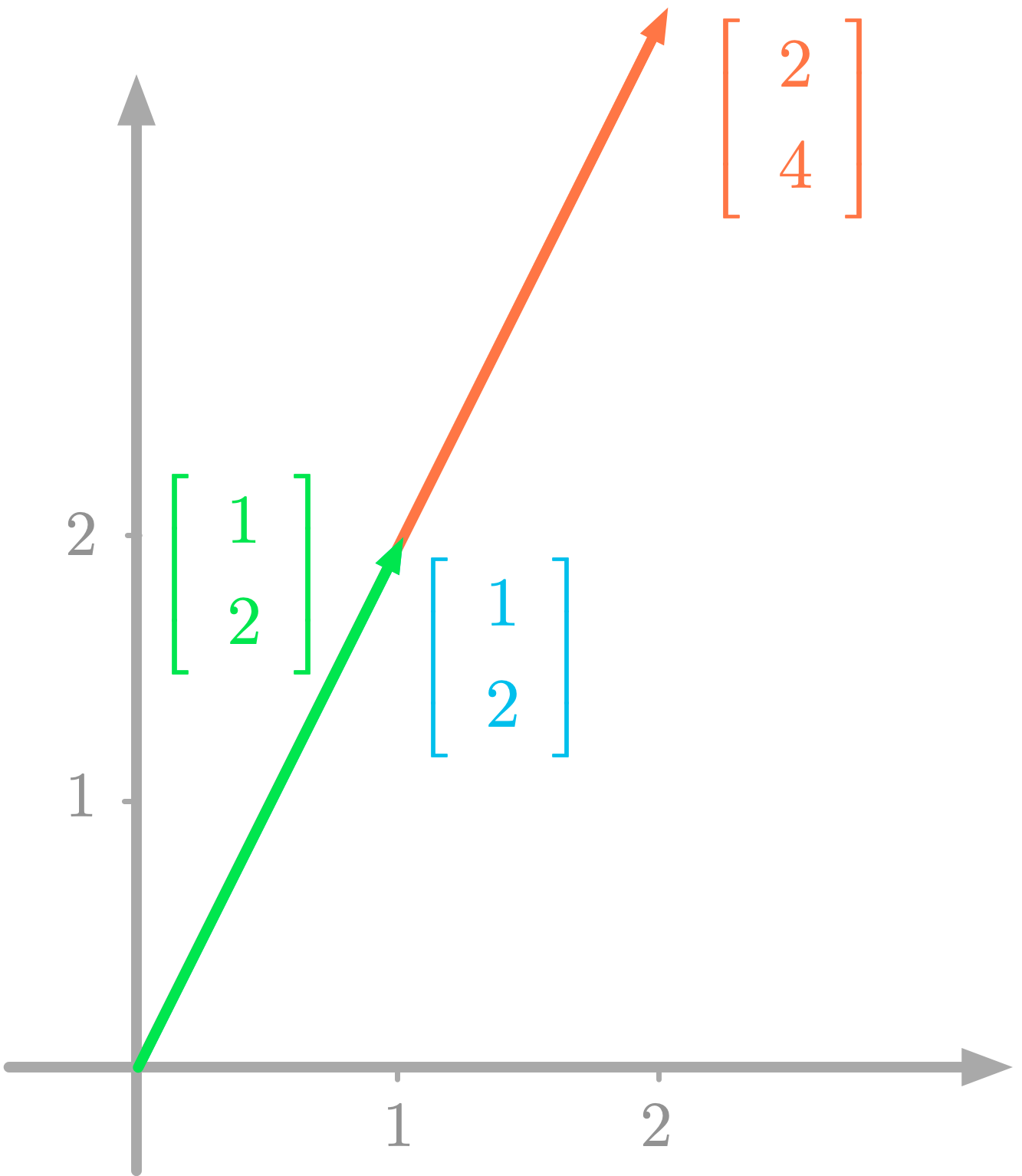 Figure 8: Column picture of a linear system with an infinite number of solutions.
Figure 8 shows the corresponding vectors graphically represented. You can see that there is an infinite number of ways to reach the endpoint of the green vector with combinations of the blue and red vectors.
Since both vectors go in the same direction, there is an infinite number of linear combinations allowing you to reach the right-hand side vector.
Summary
To summarize, you can have three possible situations, shown with two equations and two variables in Figure 9.
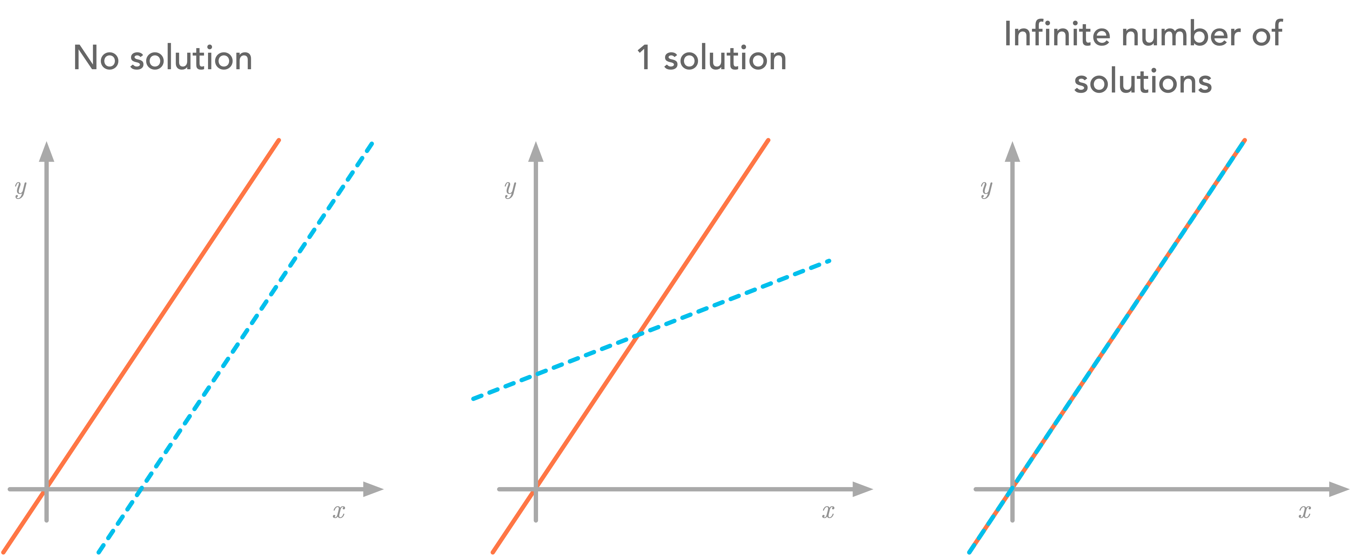 Figure 9: Summary of the three situations for two equations and two variables.
It is impossible to have two lines crossing more than once and less than an infinite number of times.
The principle holds for more dimensions. For instance, with three planes in $\setR^3$, at least two can be parallel (no solution), the three can intersect (one solution), or the three can be superposed (infinite number of solutions).
Representation of Linear Equations With Matrices
Now that you can write vector equations using the column picture, you can go further and use a matrix to store the column vectors.
Let’s take again the following linear system:
Remember from Essential Math for Data Science that you can write linear combinations as a matrix-vector product. The matrix corresponds to the two column vectors from the left-hand side concatenated:
And the vector corresponds to the coefficients weighting the column vectors of the matrix (here, $x$ and $y$):
Your linear system becomes the following matrix equation:
Notation
This leads to the following notation widely used to write linear systems:
with $\mA$ the matrix containing the column vectors, $\vx$ the vector of coefficients and $\vb$ the resulting vector, that we’ll call the target vector. It allows you to go from calculus, where equations are considered separately, to linear algebra, where every piece of the linear system are represented as vectors and matrices. This abstraction is very powerful and brings vector space theory to solve systems of linear equations.
With the column picture, you want to find the coefficients of the linear combination of the column vectors on the left-hand side of the equation. The solution exists only if the target vector is within their span.
Learn the math needed for data science and machine learning using a practical approach with Python.