
Essential Math for Data Science: The Poisson Distribution
Learn the math needed for data science and machine learning using a practical approach with Python.

The Poisson distribution, named after the French mathematician Denis Simon Poisson, is a discrete distribution function describing the probability that an event will occur a certain number of times in a fixed time (or space) interval. It is used to model count-based data, like the number of emails arriving in your mailbox in one hour or the number of customers walking into a shop in one day, for instance.
Mathematical Definition
Let’s start with an example, Figure 1 shows the number of emails received by Sarah in intervals of one hour.
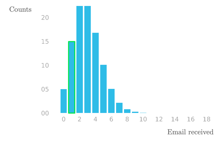 Figure 1: Emails received by Sarah in one-hour intervals for the last 100 hours.
The bar heights show the number of one-hour intervals in which Sarah observed the corresponding number of emails. For instance, the highlighted bar shows that there were around 15 one-hour slots where she received a single email.
The Poisson distribution is parametrized by the expected number of events $\lambda$ (pronounced “lambda”) in a time or space window. The distribution is a function that takes the number of occurrences of the event as input (the integer called $k$ in the next formula) and outputs the corresponding probability (the probability that there are $k$ events occurring).
The Poisson distribution, denoted as $\text{Poi}$ is expressed as follows: \[\text{Poi}(k ; \lambda) = \frac{\lambda^k e^{-\lambda}}{k!}\]
for $k=0, 1, 2, …$.
The formula of $\text{Poi}(k ; \lambda)$ returns the probability of observing $k$ events given the parameter $\lambda$ which corresponds to the expected number of occurrences in that time slot.
Note that both the binomial and the Poisson distributions are discrete: they give probabilities of discrete outcomes: the number of times an event occurs for the Poisson distribution and the number of successes for the binomial distribution. However, while the binomial calculates this discrete number for a discrete number of trials (like a number of coin toss), the Poisson considers an infinite number of trials (each trial corresponds to a very small portion of time) leading to a very small probability associated with each event.
You can refer to the section below to see how the Poisson distribution is derived from the binomial distribution.
Example
Priya is recording birds in a national park, using a microphone placed in a tree. She is counting the number of times a bird is recorded singing and wants to model the number of birds singing in a minute. For this task, she’ll assume independence of the detected birds.
Looking at the data of the last few hours, Priya observes that in average, there are two birds detected in an interval of one minute. So the value 2 could be a good candidate for the parameter of the distribution $\lambda$. Her goal is to know the probability that a specific number of birds will sing in the next minute.
Let’s implement the Poisson distribution function from the formula you saw above:
def poisson_distribution(k, lambd):
    return (lambd ** k * np.exp(-lambd)) / np.math.factorial(k)
Remember that $\lambda$ is the expected number of times a bird sings in a one-minute interval, so in this example, you have $\lambda=2$. The function poisson_distribution(k, lambd) takes the value of $k$ and $\lambda$ and returns the probability to observe $k$ occurrences (that is, to record $k$ birds singing).
For instance, the probability of Priya observing 5 birds in the next minute would be:
poisson_distribution(k=5, lambd=2)
0.03608940886309672
The probability that 5 birds will sing in the next minute is around 0.036 (3.6%).
As with the binomial function, this will overflow for larger values of $k$. For this reason, you might want to use poisson from the module scipy.stats, as follows:
from scipy.stats import poisson

poisson.pmf(5, 2)
0.03608940886309672
Let’s plot the distribution for various values of $k$:
lambd=2

k_axis = np.arange(0, 25)
distribution = np.zeros(k_axis.shape[0])
for i in range(k_axis.shape[0]):
    distribution[i] = poisson.pmf(i, lambd)

plt.bar(k_axis, distribution)
# [...] Add axes, labels...
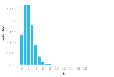 Figure 2: Poisson distribution for $\lambda=2$.
The probabilities corresponding to the values of $k$ are summarized in the probability mass function shown in Figure
- You can see that it is most probable that Priya will hear one or two birds singing in the next minute.
Finally, you can plot the function for different values of $\lambda$:
f, axes = plt.subplots(6, figsize=(6, 8), sharex=True)

for lambd in range(1, 7):

    k_axis = np.arange(0, 20)
    distribution = np.zeros(k_axis.shape[0])
    for i in range(k_axis.shape[0]):
        distribution[i] = poisson.pmf(i, lambd)

    axes[lambd-1].bar(k_axis, distribution)
    axes[lambd-1].set_xticks(np.arange(0, 20, 2))
    axes[lambd-1].set_title(f"$\lambda$: {lambd}")

# Add axes labels etc.
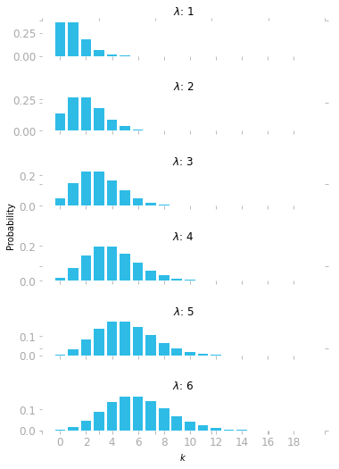 Figure 3: Poisson distribution for various values of $\lambda$.
Figure 3 shows the Poisson distribution for various values of $\lambda$, which looks a bit like a normal distribution in some cases. However, the Poisson distribution is discrete, not symmetric when the value of $\lambda$ is low, and bounded to zero.
Bonus: Deriving the Poisson Distribution
Let’s see how the Poisson distribution is derived from the Binomial distribution.
You saw in Essential Math for Data Science that if you run a random experiment multiple times, the probability to get $m$ successes over $N$ trials, with a probability of a success $\mu$ at each trial, is calculated through the binomial distribution: \[\text{Bin}(k ;N, \mu) = \binom{N}{k} \mu^k (1-\mu)^{N-k}\]
Problem Statement
How can you use the binomial formula to model the probability to observe an event a certain number of times in a given time interval instead of in a certain number of trials? There are a few problems:
You don’t know $N$, since there is no specific number of trials, only a time window.
You don’t know $\mu$, but you have the expected number of times the event will occur. For instance, you know that in the past 100 hours, you received an average of 3 emails per hour, and you want to know the probability of receiving 5 emails in the next hour.
Let’s handle these issues mathematically.
To address the first point, you can consider time as small discrete chunks. Let’s call these chunck $\epsilon$ (pronounced “epsilon”), as shown in Figure 4. If you consider each chunk as a trial, you have $N$ chunks.
 Figure 4: You can split the continuous time in segments of length $\epsilon$.
The estimation of a continuous time scale is more accurate when $\epsilon$ is very small. If $\epsilon$ is small, the number of segments $N$ will be large. In addition, since the segments are small, the probability of success in each segment is also small.
To summarize, you want to modify the binomial distribution to be able model a very large number of trials, each with a very small probability of success. The trick is to consider that $N$ tends toward infinity (because continuous time is approximated by having a value of $\epsilon$ that tends toward zero).
Update the Binomial Formula
Let’s find $\mu$ in this case and replace it in the binomial formula. You know the expected number of event in a period of time $t$, which we’ll call $\lambda$ (pronounced “lambda”). Since you split $t$ into small intervals of length $\epsilon$, you have the number of trials: \[N=t \cdot \epsilon\]
You have $\lambda$ as the number of successes in the $N$ trials. So the probability $\mu$ to have a success in one trial is: \[\mu = \frac{\lambda}{N}\]
Replacing $\mu$ in the binomial formula, you get: \[\binom{N}{k} \left(\frac{\lambda}{N} \right)^k \left(1 - \frac{\lambda}{N} \right)^{N-k}\]
Developing the expression, writing the binomial coefficient as factorials (as you did in Essential Math for Data Science), and using the fact $a^{b-c}=a^b-a^c$, you have: \[\frac{N!}{(N-k)!k!} \left(\frac{\lambda}{N} \right)^k \left(1 - \frac{\lambda}{N} \right)^{N} \left(1 - \frac{\lambda}{N} \right)^{-k}\]
Let’s consider the first element of this expression. If you state that $N$ tends toward infinity (because $\epsilon$ tends toward zero), you have: \[\lim_{N \to +\infty} \frac{N!}{(N-k)!} = N^k\]
This is because $k$ can be ignored when it is small in comparison to $N$. For instance, you have: \[\frac{1,000,000!}{(1,000,000-3)!} = 1,000,000 \cdot 999,999 \cdot 999,998\]
which approximates $1,000,000 \cdot 1,000,000 \cdot 1,000,000$
So you the first ratio becomes: \[\frac{N!}{(N-k)!k!} = N^k \cdot \frac{1}{k!}\]
Then, using the fact that $\lim_{N \to +\infty}(1+\frac{\lambda}{N})^N=e^{\lambda}$, you have: \[\lim_{N \to +\infty} \left(1 - \frac{\lambda}{N} \right)^{N} = e^{-\lambda}\]
Finally, since $\left(1- \frac{\lambda}{N} \right)$ tends toward 1 when $N$ tends toward the infinity: \[\lim_{N \to +\infty} \left(1- \frac{\lambda}{N} \right)^{-k} = 1^{-k} = 1\]
Let’s replace all of this in the formula of the binomial distribution: \[\begin{aligned} &\lim_{N \to +\infty} \frac{N!}{(N-k)!k!} \left(\frac{\lambda}{N} \right)^k \left(1 - \frac{\lambda}{N} \right)^{N} \left(1 - \frac{\lambda}{N} \right)^{-k} \\\\ &= \lim_{N \to +\infty} N^k \cdot \frac{1}{k!} \cdot \left(\frac{\lambda}{N} \right)^k \cdot e^{-\lambda} \cdot 1 \\\\ &= \lim_{N \to +\infty} \frac{1}{k!} \cdot \left(N\frac{\lambda}{N} \right)^k \cdot e^{-\lambda} \\\\ &= \frac{1}{k!} \cdot \lambda^k \cdot e^{-\lambda} \\\\ &= \frac{\lambda^k e^{-\lambda}}{k!} \\\\ \end{aligned}\]
This is the Poisson distribution, denoted as $\text{Poi}$: \[\text{Poi}(k ; \lambda) = \frac{\lambda^k e^{-\lambda}}{k!}\]
for $k=0, 1, 2, …$.
Learn the math needed for data science and machine learning using a practical approach with Python.