
Essential Math for Data Science: Probability Density and Probability Mass Functions
Learn the math needed for data science and machine learning using a practical approach with Python.
In the chapter 02 of Essential Math for Data Science, you can learn about basic descriptive statistics and probability theory. We’ll cover probability mass and probability density function in this sample. You’ll see how to understand and represent these distribution functions and their link with histograms.
Deterministic processes give the same results when they are repeated multiple times. This is not the case for random variables, which describe stochastic events, in which randomness characterizes the process.
This means that random variables can take various values. How can you describe and compare these values? One good way is to use the probability that each outcome will occur. The probability distribution of a random variable is a function that takes the sample space as input and returns probabilities: in other words, it maps possible outcomes to their probabilities.
In this section, you’ll learn about probability distributions for discrete and continuous variables.
Probability Mass Functions
Probability functions of discrete random variables are called probability mass functions (or PMF). For instance, let’s say that you’re running a dice-rolling experiment. You call $\rx$ the random variable corresponding to this experiment. Assuming that the die is fair, each outcome is equiprobable: if you run the experiment a large number of times, you will get each outcome approximately the same number of times. Here, there are six possible outcomes, so you have one chance over six to draw each number.
Thus, the probability mass function describing $\rx$ returns $\frac{1}{6}$ for each possible outcome and 0 otherwise (because you can’t get something different than 1, 2, 3, 4, 5 or 6).
You can write $P(\rx = 1) = \frac{1}{6}$, $P(\rx = 2) = \frac{1}{6}$, and so on.
Properties of Probability Mass Functions
Not every function can be considered as a probability mass function. A probability mass function must satisfy the following two conditions:
- The function must return values between 0 and 1 for each possible outcome:
- The sum of probabilities corresponding to all the possible outcomes must be equal to 1:
The value of $x$ can be any real number because values outside of the sample space are associated with a probability of 0. Mathematically, for any value $x$ not in the sample space $S$, $P(x)=0$.
Simulation of the Dice Experiment
Let’s simulate a die experiment using the function np.random.randint(low, high, size) from Numpy which draw $n$ (size) random integers between low and high (excluded). Let’s simulate 20 die rolls:
rolls = np.random.randint(1, 7, 20)
rolls
array([6, 3, 5, ..., 6, 5, 1])
This array contains the 20 outcomes of the experiment. Let’s call $\rx$ the discrete random variable corresponding to the die rolling experiment. The probability mass function of $\rx$ is defined only for the possible outcomes and gives you the probability for each of them.
Assuming the die is fair, you should have an uniform distribution, that is, equiprobable outcomes..
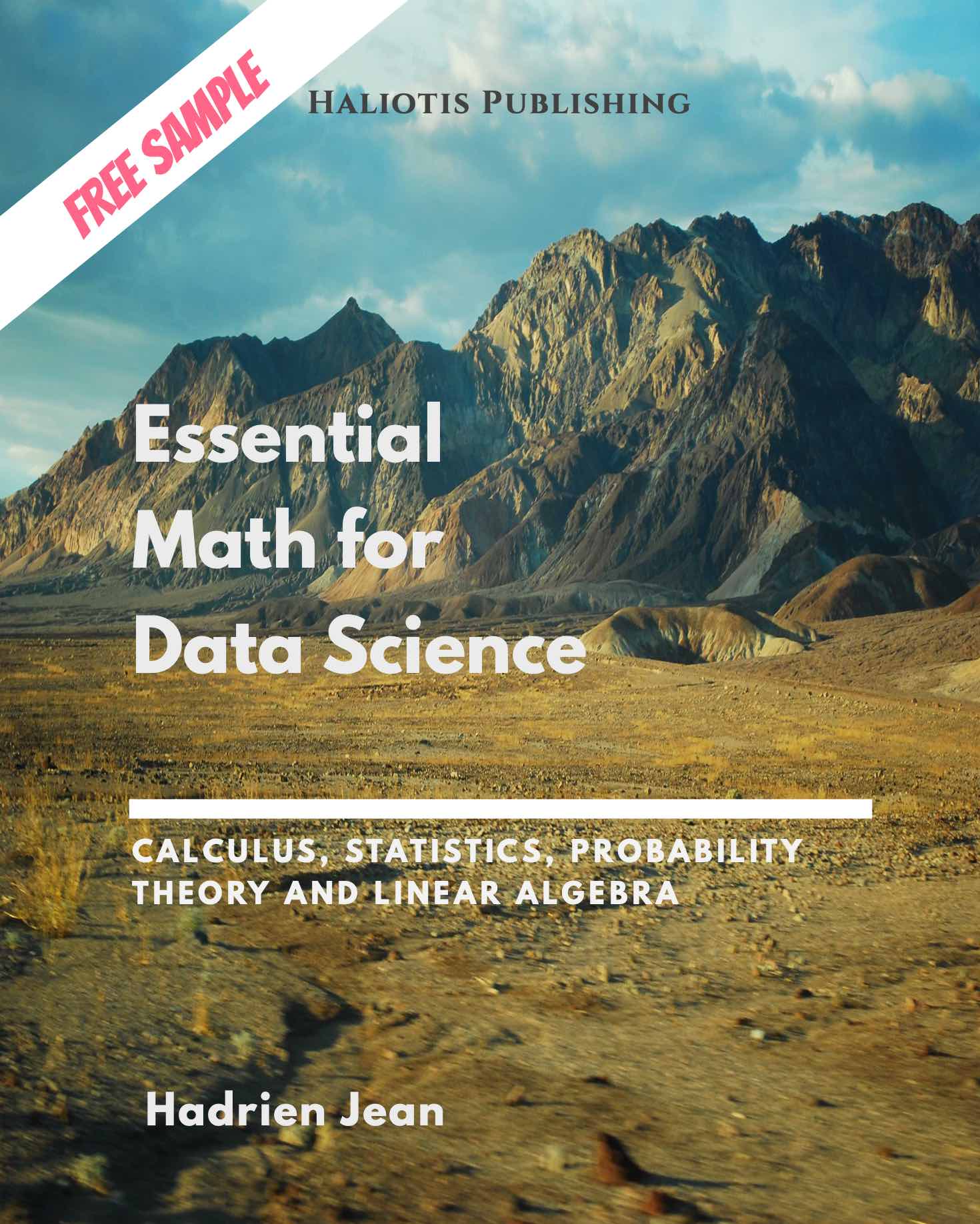
Let’s visualize the quantity of each outcome you got in the random experiment. You can divide by the number of trials to get the probability. Let’s use plt.stem() from Matplotlib to visualize these probabilities:
val, counts = np.unique(rolls, return_counts=True)
plt.stem(val, counts/len(rolls), basefmt="C2-", use_line_collection=True)
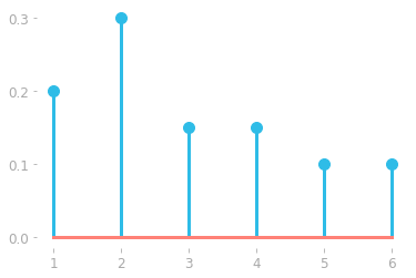 Figure 1: Probability mass function of the random variable $\rx$ corresponding to a die rolling a six-sided die estimated from 20 rolls.
With a uniform distribution, the plot would have the same height for each outcome (since the height corresponds to the probability, which is the same for each outcome of a die throw). However, the distribution shown in Figure 1 doesn’t look uniform. That’s because you didn’t repeat the experiment enough: the probabilities will stand when you repeat the experiment a large number of times (in theory, an infinite number of times).
Let’s increase the number of trials:
throws = np.random.randint(1, 7, 100000)
val, counts = np.unique(throws, return_counts=True)
plt.stem(val, counts/len(throws), basefmt="C2-", use_line_collection=True)
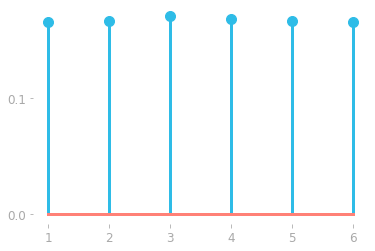 Figure 2: Probability mass function of the random variable $\rx$ corresponding to a die rolling experiment estimated from 100,000 rolls.
With enough trials, the probability mass function showed in Figure 2 looks uniform. This underline the importance of the number of trials from a frequentist probability point of view.
Probability Density Functions
With continuous variables, there is an infinite number of possible outcomes (limited by the number of decimals you use). For instance, if you were drawing a number between 0 and 1 you might get an outcome of, for example, 0.413949834. The probability of drawing each number tends towards zero: if you divide something by a very large number (the number of possible outcomes), the result will be very small, close to zero. This is not very helpful in describing random variables.
It is better to consider the probability of getting a specific number within a range of values. The $y$-axis of probability density functions is not a probability. It is called a probability density or just density. Thus, probability distributions for continuous variables are called probability density functions (or PDF).
The integral of the probability density function over a particular interval gives you the probability that a random variable takes a value in this interval. This probability is thus given by the area under the curve in this interval (as you can see in Essential Math for Data Science).
Notation
Here, I’ll denote probability density functions using a lowercase $p$. For instance, the function $p(x)$ gives you the density corresponding to the value $x$.
Example
Let’s inspect an example of probability density function. You can randomly draw data from a normal distribution using the Numpy function np.random.normal (you’ll find more details about the normal distribution in Essential Math for Data Science).
You can choose the parameters of the normal distribution (the mean and the standard deviation) and the number of samples. Let’s create a variable data with 1,000 values drawn randomly from a normal distribution with a mean of 0.3 and a standard deviation of 0.1.
np.random.seed(123)
data = np.random.normal(0.3, 0.1, 1000)
Let’s look at the shape of the distribution using an histogram. The function plt.hist() returns the exact values for the $x$- and $y$-coordinates of the histogram. Let’s store this in a variable called hist for latter use:
hist = plt.hist(data, bins=13, range=(-0.3, 1))
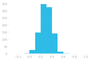 Figure 3: Histogram of the data generated from a normal distribution. The $x$-axis is the value of the element in the vector and the $y$-axis the number of elements (count) that are in the corresponding range.
Histograms
bins in the function hist()).
For instance, Figure 3 shows that there are around 347 elements in the interval (0.2, 0.3). Each bin corresponds to a width of 0.1, since we used 13 bins to represent data in the range -0.3 to 1.
Let’s have a closer look at the distribution with more bins. You can use the parameter density to make the $y$-axis correspond to the probability density instead of the count of values in each bin:
hist = plt.hist(data, bins=24, range=(-0.2, 1), density=True)
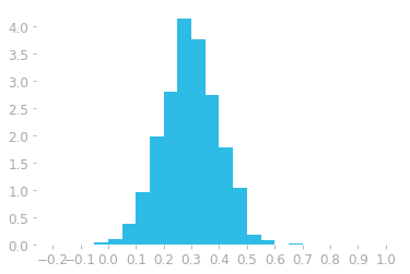 Figure 4: Histogram using 30 bins and density instead of counts.
You can see in Figure 4 that there are more bins in this histogram (24 instead of 13). This means that each bin has now a smaller width. The $y$-axis is also on a different scale: it corresponds to the density, not the counter of values as before.
To calculate the probability to draw a value in a certain range from the density, you need to use the area under the curve. In the case of histograms, this is the area of the bars.
Let’s take an example with the bar ranging from 0.2 to 0.25, associated with the following density:
print(f"Density: {hist[0][8].round(4)}")
print(f"Range x: from {hist[1][8].round(4)} to {hist[1][9].round(4)}")
Density: 2.8
Range x: from 0.2 to 0.25
Since there are 24 bins and the range of possible outcomes is from -0.2 to 1, each bar corresponds to a range of $\frac{1-(-0.2)}{24}=\frac{1.2}{24}=0.05$. In our example, the height of the bar (the one from 0.2 to 0.25) is around 2.8, so the area of this bar is $2.8 \cdot 0.05 = 0.14$. This means that the probability of getting a value between 0.2 and 0.25 is around 0.14, or 14%.
You saw that the sum of the probabilities must be equal to one, so the sum of the bar’s areas should be equal to one. Let’s check that: you can take the vector containing the densities (hist[0]) and multiply it by the bar width (0.05):
(hist[0] * 0.05).sum().round(4)
1.0
All good: the sum of the probabilities is equal to one.
From Histograms to Continuous Probability Density Functions
Histograms represent a binned version of the probability density function. Figure 5 shows a representation of the true probability density function. The blue shaded area in the figure corresponds to the probability of getting a number between 0 and 0.2 (the area under the curve between 0 and 0.2).
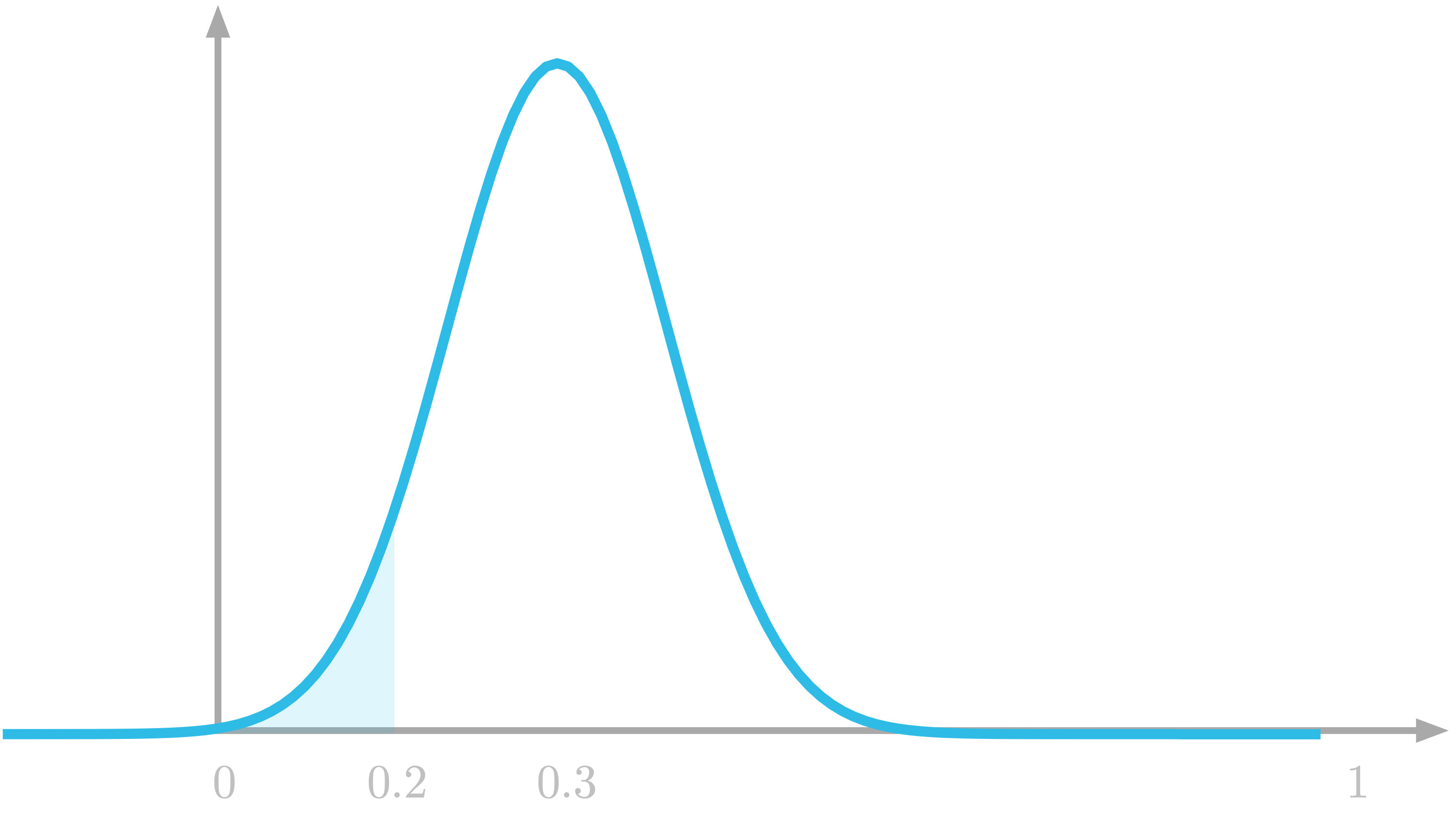 Figure 5: The probability to draw a number between 0 and 0.2 is the highlighted area under the curve.
Properties of Probability Density Functions
Like probability mass functions, probability density functions must satisfy some requirements. The first is that it must return only non negative values. Mathematically written: \[p(x) \geq 0\]
The second requirement is that the total area under the curve of the probability density function must be equal to 1: \[\int_{-\infty}^{\infty} p(x) \; dx = 1\]
In this part on probability distributions, you saw that probability mass functions are for discrete variables and probability density functions for continuous variables. Keep in mind that the value on the $y$ axis of probability mass functions are probabilities, which is not the case for probability density functions. Look at the density values (for instance in Figure 4): they can be larger than one, which shows that they are not probabilities.
Learn the math needed for data science and machine learning using a practical approach with Python.