
Essential Math for Data Science: Basis and Change of Basis
Learn the math needed for data science and machine learning using a practical approach with Python.

Basis and Change of Basis
One way to understand eigendecomposition is to consider it as a change of basis. You’ll learn in this article what is the basis of a vector space.
You’ll see that any vector of the space are linear combinations of the basis vectors and that the number you see in vectors depends on the basis you choose.
Finally, you’ll see how to change the basis using change of basis matrices.
It is a nice way to consider matrix factorization as eigendecomposition or Singular Value Decomposition. As you can see in Chapter 09 of Essential Math for Data Science, with eigendecomposition, you choose the basis such that the new matrix (the one that is similar to the original matrix) becomes diagonal.
Definitions
The basis is a coordinate system used to describe vector spaces (sets of vectors). It is a reference that you use to associate numbers with geometric vectors.
To be considered as a basis, a set of vectors must:
- Be linearly independent.
- Span the space.
Every vector in the space is a unique combination of the basis vectors. The dimension of a space is defined to be the size of a basis set. For instance, there are two basis vectors in $\setR^2$ (corresponding to the $x$ and $y$-axis in the Cartesian plane), or three in $\setR^3$.
As shown in section 7.4 of Essential Math for Data Science, if the number of vectors in a set is larger than the dimensions of the space, they can’t be linearly independent. If a set contains fewer vectors than the number of dimensions, these vectors can’t span the whole space.
As you saw, vectors can be represented as arrows going from the origin to a point in space. The coordinates of this point can be stored in a list. The geometric representation of a vector in the Cartesian plane implies that we take a reference: the directions given by the two axes $x$ and $y$.
Basis vectors are the vectors corresponding to this reference. In the Cartesian plane, the basis vectors are orthogonal unit vectors (length of one), generally denoted as $\vi$ and $\vj$.
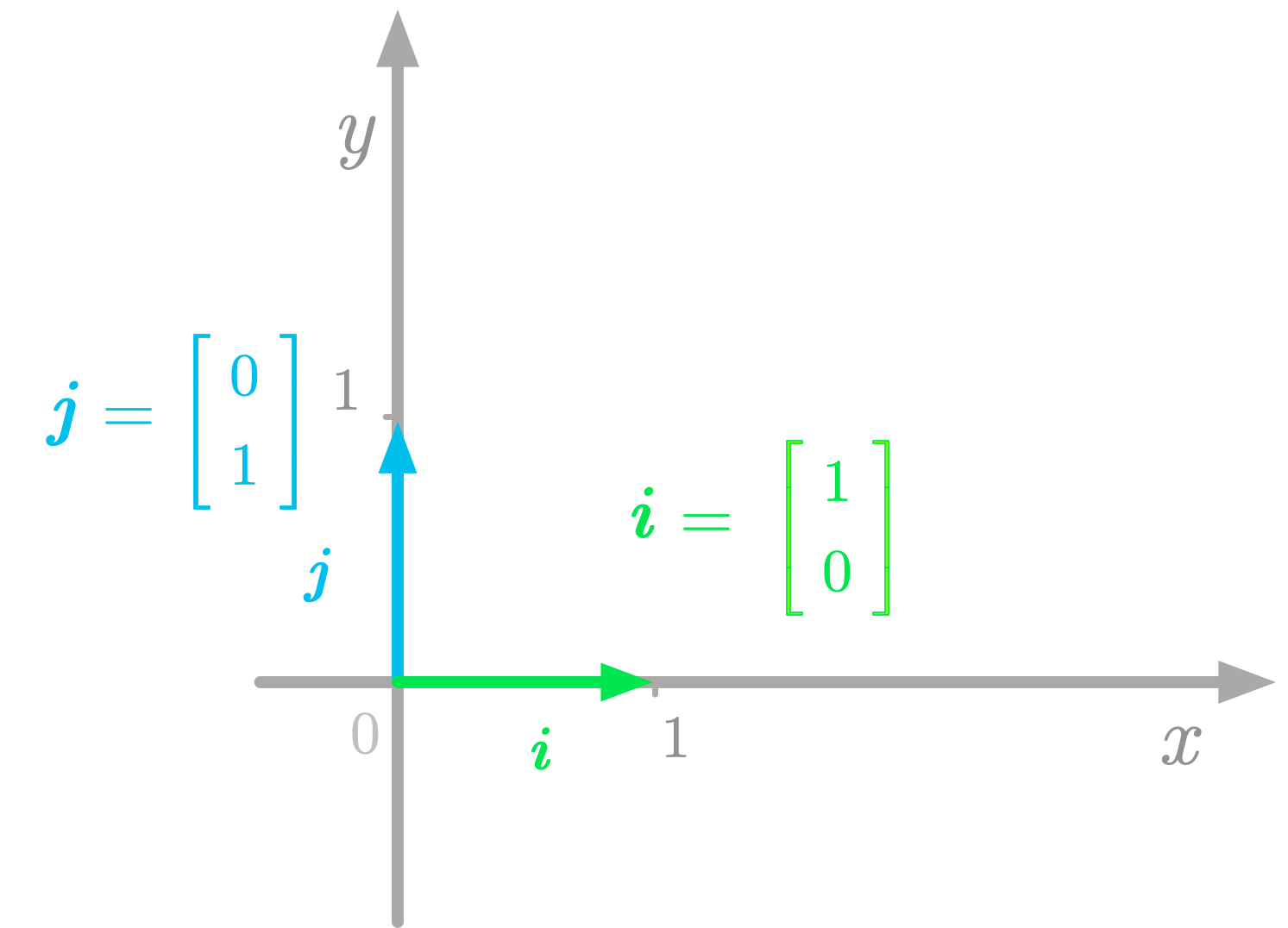 Figure 1: The basis vectors in the Cartesian plane.
For instance, in Figure 1, the basis vectors $\vi$ and $\vj$ point in the direction of the $x$-axis and $y$-axis respectively. These vectors give the standard basis. If you put these basis vectors into a matrix, you have the following identity matrix (for more details about identity matrices, see 6.4.3 in Essential Math for Data Science):
Thus, the columns of $\mI_2$ span $\setR^2$. In the same way, the columns of $\mI_3$ span $\setR^3$ and so on.
Basis vectors can be orthogonal because orthogonal vectors are independent. However, the converse is not necessarily true: non-orthogonal vectors can be linearly independent and thus form a basis (but not a standard basis).
The basis of your vector space is very important because the values of the coordinates corresponding to the vectors depend on this basis. By the way, you can choose different basis vectors, like in the ones in Figure 2 for instance.
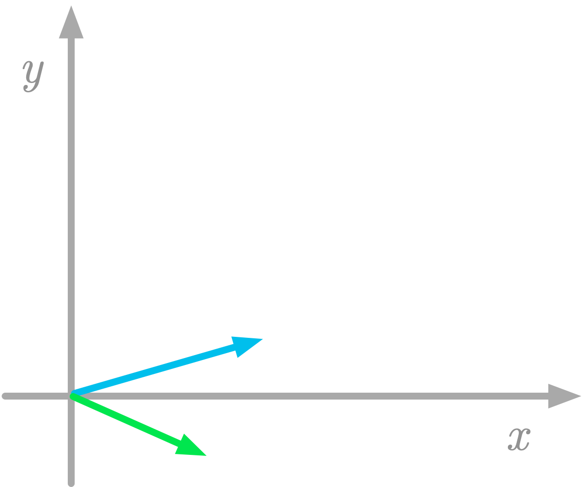 Figure 2: Another set of basis vectors.
Keep in mind that vector coordinates depend on an implicit choice of basis vectors.
Linear Combination of Basis Vectors
You can consider any vector in a vector space as a linear combination of the basis vectors.
For instance, take the following two-dimensional vector $\vv$:
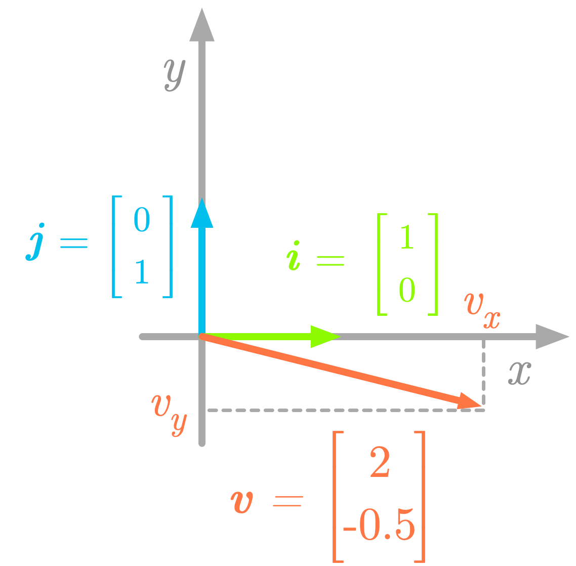 Figure 3: Components of the vector $\vv$.
The components of the vector $\vv$ are the projections on the $x$-axis and on the $y$-axis ($\evv_x$ and $\evv_y$, as illustrated in Figure 3). The vector $\vv$ corresponds to the sum of its components: $\vv = \evv_x + \evv_y$, and you can obtain these components by scaling the basis vectors: $\evv_x = 2 \vi$ and $\evv_y = -0.5 \vj$. Thus, the vector $\vv$ shown in Figure 3 can be considered as a linear combination of the two basis vectors $\vi$ and $\vj$:
Other Bases
The columns of identity matrices are not the only case of linearly independent columns vectors. It is possible to find other sets of $n$ vectors linearly independent in $\setR^n$.
For instance, let’s consider the following vectors in $\setR^2$:
and
The vectors $\vv$ and $\vw$ are represented in Figure 4.
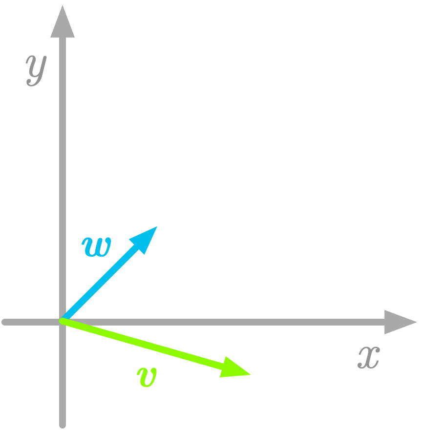 Figure 4: Another basis in a two-dimensional space.
From the definition above, the vectors $\vv$ and $\vw$ are a basis because they are linearly independent (you can’t obtain one of them from combinations of the other) and they span the space (all the space can be reached from the linear combinations of these vectors).
It is critical to keep in mind that, when you use the components of vectors (for instance $\evv_x$ and $\evv_y$, the $x$ and $y$ components of the vector $\vv$), the values are relative to the basis you chose. If you use another basis, these values will be different.
You can see in Chapter 09 and 10 of Essential Math for Data Science that the ability to change the bases is fundamental in linear algebra and is key to understand eigendecomposition or Singular Value Decomposition.
Vectors Are Defined With Respect to a Basis
You saw that to associate geometric vectors (arrows in the space) with coordinate vectors (arrays of numbers), you need a reference. This reference is the basis of your vector space. For this reason, a vector should always be defined with respect to a basis.
Let’s take the following vector:
The values of the $x$ and $y$ components are respectively 2 and -0.5. The standard basis is used when not specified.
You could write $\mI \vv$ to specify that these numbers correspond to coordinates with respect to the standard basis. In this case $\mI$ is called the change of basis matrix.
You can define vectors with respect to another basis by using another matrix than $\mI$.
Linear Combinations of the Basis Vectors
Vector spaces (the set of possible vectors) are characterized in reference to a basis. The expression of a geometrical vector as an array of numbers implies that you choose a basis. With a different basis, the same vector $\vv$ is associated with different numbers.
You saw that the basis is a set of linearly independent vectors that span the space. More precisely, a set of vectors is a basis if every vector from the space can be described as a finite linear combination of the components of the basis and if the set is linearly independent.
Consider the following two-dimensional vector:
In the $\setR^2$ Cartesian plane, you can consider $\vv$ as a linear combination of the standard basis vectors $\vi$ and $\vj$, as shown in Figure 5.
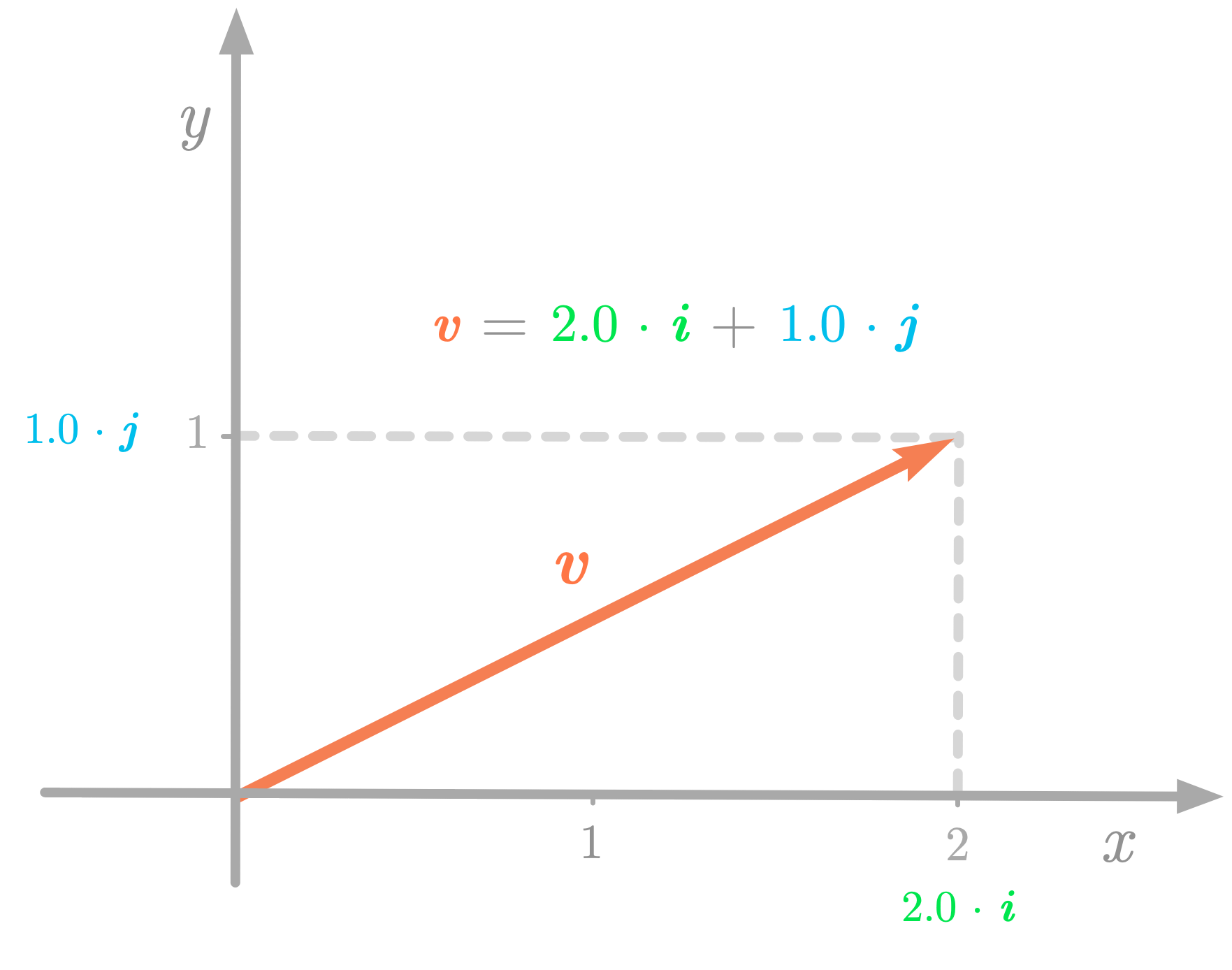 Figure 5: The vector $\vv$ can be described as a linear combination of the basis vectors $\vi$ and $\vj$.
But if you use another coordinate system, $\vv$ is associated with new numbers. Figure 6 shows a representation of the vector $\vv$ with a new coordinate system ($\vi’$ and $\vj’$).
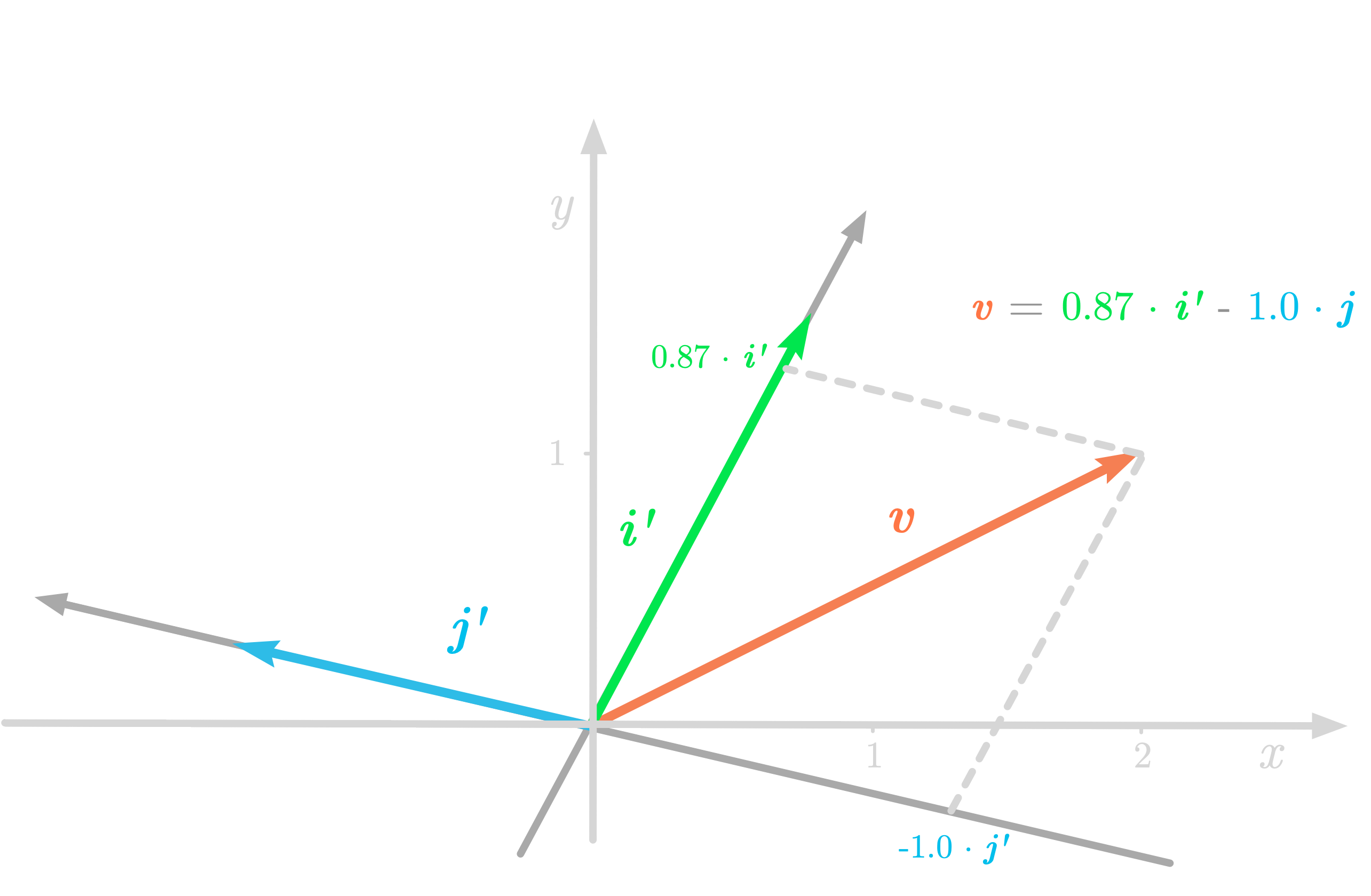 Figure 6: The vector $\vv$ with respect to the coordinates of the new basis.
In the new basis, $\vv$ is a new set of numbers:
The Change of Basis Matrix
You can use a change of basis matrix to go from a basis to another. To find the matrix corresponding to new basis vectors, you can express these new basis vectors ($\vi’$ and $\vj’$) as coordinates in the old basis ($\vi$ and $\vj$).
Let’s take again the preceding example. You have:
and
This is illustrated in Figure 7.
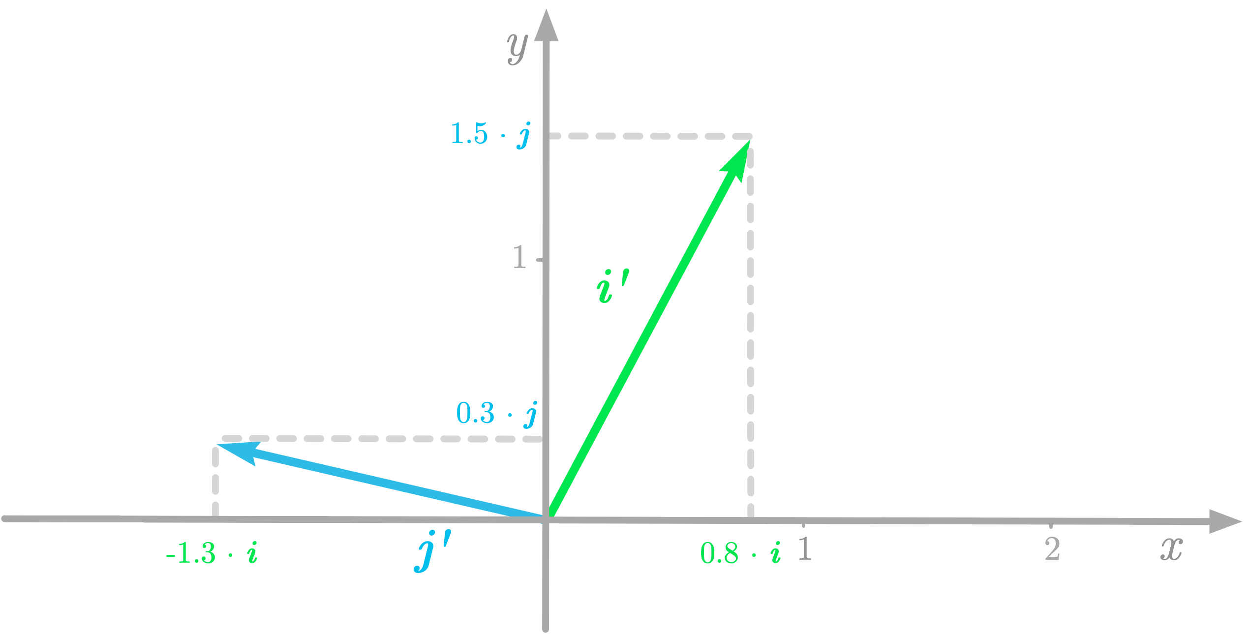 Figure 7: The coordinates of the new basis vectors with respect to the old basis.
Since they are basis vectors, $\vi’$ and $\vj’$ can be expressed as linear combinations of $\vi$ and $\vj$.:
Let’s write these equations under the matrix form:
To have the basis vectors as columns, you need to transpose the matrices. You get:
This matrix is called the change of basis matrix. Let’s call it $\mC$:
As you can notice, each column of the change of basis matrix is a basis vector of the new basis. You’ll see next that you can use the change of basis matrix $\mC$ to convert vectors from the output basis to the input basis.
Finding the Change of Basis Matrix
A change of basis matrix maps an input basis to an output basis. Let’s call the input basis $\mB_1$ with the basis vectors $\vi$ and $\vj$, and the output basis $\mB_2$ with the basis vectors $\vi’$ and $\vj’$. You have:
and
From the equation of the change of basis, you have:
If you want to find the change of basis matrix given $\mB_1$ and $\mB_2$, you need to calculate the inverse of $\mB_1$ to isolate $\mC$:
In words, you can calculate the change of basis matrix by multiplying the inverse of the input basis matrix ($\mB_1^{-1}$, which contains the input basis vectors as columns) by the output basis matrix ($\mB_2$, which contains the output basis vectors as columns).
Note that if the input basis is the standard basis ($\mB_1=\mI$), then the change of basis matrix is simply the output basis matrix:
Since the basis vectors are linearly independent, the columns of $\mC$ are linearly independent, and thus, as stated in section 7.4 of Essential Math for Data Science, $\mC$ is invertible.
Example: Changing the Basis of a Vector
Let’s change the basis of a vector $\vv$, using again the geometric vectors represented in Figure 6.
Notation
You’ll change the basis of $\vv$ from the standard basis to a new basis. Let’s denote the standard basis as $\mB_1$ and the new basis as $\mB_2$. Remember that the basis is a matrix containing the basis vectors as columns. You have:
and
Let’s denote the vector $\vv$ relative to the basis $\mB_1$ as $\lbrack \vv \rbrack_{\mB_1}$:
The goal is to find the coordinates of $\vv$ relative to the basis $\mB_2$, denoted as $\lbrack \vv \rbrack_{\mB_2}$.
To distinguish the basis used to define a vector, you can put the basis name (like $\mB_1$) in subscript after the vector name enclosed in square brackets. For instance, $\lbrack \vv \rbrack_{\mB_1}$ denotes the vector $\vv$ relative to the basis $\mB_1$, also called the representation of $\vv$ with respect to $\mB_1$.
Using Linear Combinations
Let’s express the vector $\vv$ as a linear combination of the input and output basis vectors:
The scalars $c_1$ and $c_2$ are weighting the linear combination of the input basis vectors, and the scalars $d_1$ and $d_2$ are weighting the linear combination of the output basis vectors. You can merge the two equations:
Now, let’s write this equation in matrix form:
The vector containing the scalars $c_1$ and $c_2$ corresponds to $\lbrack \vv \rbrack_{\mB_1}$ and the vector containing the scalars $d_1$ and $d_2$ corresponds to $\lbrack \vv \rbrack_{\mB_2}$. You have:
That’s good, this an equation with the term you want to find: $\lbrack \vv \rbrack_{\mB_2}$. You can isolate it by multiplying each side by $\mB_2 ^ {-1}$:
You have also:
The term $\mB_2 ^ {-1} \mB_1$ is the inverse of $\mB_1 ^ {-1} \mB_2$, which is the change of basis matrix $\mC$ described before. This shows that $\mC^{-1}$ allows you to convert vectors from an input basis $\mB_1$ to an output basis $\mB_2$ and $\mC$ from $\mB_2$ to $\mB_1$.
In the context of this example, since $\mB_1$ is the standard basis, it simplifies to:
This means that, applying the matrix $\mB_2 ^ {-1}$ to $\lbrack \vv \rbrack_{\mB_1}$ allows you to change its basis to $\mB_2$.
Let’s code this:
v_B1 = np.array([2, 1])
B_2 = np.array([
    [0.8, -1.3],
    [1.5, 0.3]
])

v_B2 = np.linalg.inv(B_2) @ v_B1
v_B2
array([ 0.86757991, -1.00456621])
These values are the coordinates of the vector $\vv$ relative to the basis $\mB_2$. This means that if you go to $0.86757991 \vi’ - 1.00456621 \vj’$ you arrive to the position (2, 1) in the standard basis, as illustrated in Figure 6.
Conclusion
Understanding the concept of basis is a nice way to approach matrix decomposition (also called matrix factorization), like eigendecomposition or singular value decomposition (SVD). In these terms, you can think of matrix decomposition as finding a basis where the matrix associated with a transformation has specific properties: the factorization is a change of basis matrix, the new transformation matrix, and finally the inverse of the change of basis matrix to come back into the initial basis (more details in Chapter 09 and 10 of Essential Math for Data Science).
Learn the math needed for data science and machine learning using a practical approach with Python.